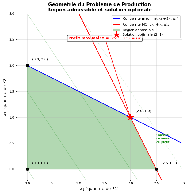
# Visualisation geometrique du probleme de production
fig, ax = plt.subplots(figsize=(10, 8))

# Domaine de tracage
x = np.linspace(0, 3, 400)

# Contrainte 1: x1 + 2*x2 <= 4 => x2 <= (4 - x1) / 2
y1 = (4 - x) / 2

# Contrainte 2: 2*x1 + x2 <= 5 => x2 <= 5 - 2*x1
y2 = 5 - 2 * x

# Tracer les contraintes
ax.plot(x, y1, 'b-', linewidth=2, label=r'Contrainte machine: $x_1 + 2x_2 \leq 4$')
ax.plot(x, y2, 'r-', linewidth=2, label=r'Contrainte MO: $2x_1 + x_2 \leq 5$')

# Region admissible (intersection des contraintes)
y_feasible = np.minimum(y1, y2)
ax.fill_between(x, 0, y_feasible, where=(y_feasible >= 0),
                   alpha=0.3, color='green', label='Region admissible')

# Sommets du polyedre (intersections des contraintes + axes) :
#   (0,0)   : origine (axes x1>=0 et x2>=0)
#   (0,2)   : axe x1=0  sur la contrainte machine  (0+2*2=4)
#   (2,1)   : intersection machine ∩ MO  (2+2*1=4 ET 2*2+1=5)  <- OPTIMAL
#   (2.5,0) : axe x2=0  sur la contrainte MO      (2*2.5+0=5)
vertices = [(0, 0), (0, 2), (2, 1), (2.5, 0)]
for vx, vy in vertices:
    ax.plot(vx, vy, 'ko', markersize=8)
    ax.text(vx + 0.1, vy + 0.1, f'({vx:.1f}, {vy:.1f})', fontsize=10)

# Solution optimale (2, 1)
ax.plot(2, 1, 'r*', markersize=20, label='Solution optimale (2, 1)')

# Courbes de niveau de la fonction objectif
for z_val in [0, 3, 6, 9]:
    y_obj = (z_val - 3 * x) / 2
    ax.plot(x, y_obj, 'g--', alpha=0.3, linewidth=1)
ax.text(2.5, 0.5, 'Courbes\nde niveau\ndu profit', fontsize=9, color='green')

# Annotation de la solution
ax.annotate('Profit maximal: z = 3*2 + 2*1 = 8€',
             xy=(2, 1), xytext=(0.8, 2.5),
             arrowprops=dict(arrowstyle='->', color='red', lw=1.5),
             fontsize=11, color='red', fontweight='bold',
             bbox=dict(boxstyle='round', facecolor='white', alpha=0.8))

# Mise en forme
ax.set_xlabel('$x_1$ (quantite de P1)', fontsize=12)
ax.set_ylabel('$x_2$ (quantite de P2)', fontsize=12)
ax.set_title('Geometrie du Probleme de Production\nRegion admissible et solution optimale',
             fontsize=14, fontweight='bold')
ax.legend(loc='upper right', fontsize=10)
ax.grid(True, alpha=0.3)
ax.set_xlim(-0.2, 3)
ax.set_ylim(-0.2, 3)
ax.set_aspect('equal')

plt.tight_layout()
plt.show()

print("Visualisation geometrique du probleme de production")
print("\nSommets de la region admissible (et profit z = 3*x1 + 2*x2) :")
print("  (0, 0)   : Profit = 3*0 + 2*0   = 0")
print("  (0, 2)   : Profit = 3*0 + 2*2   = 4")
print("  (2, 1)   : Profit = 3*2 + 2*1   = 8   <- OPTIMAL")
print("    Machine: 2 + 2*1 = 4 <= 4 (saturee) | MO: 2*2 + 1 = 5 <= 5 (saturee)")
print("  (2.5, 0) : Profit = 3*2.5 + 2*0 = 7.5")
print("    Machine: 2.5 + 2*0 = 2.5 <= 4 | MO: 2*2.5 + 0 = 5 <= 5 (saturee)")
print("\nSolution optimale : x1=2, x2=1, Profit = 8 (sommet Machine ∩ MO)")
print("(Confirme par le solveur PuLP/CBC cellule suivante.)")