Objectif
Reproduire l’analyse exploratoire de research.ipynb avec les données natives QuantConnect.
Ce notebook vs main.py — divergence assumée (C.4)
Ce quantbook est une baseline pédagogique inverse-vol simplifiée (5 ETF, sans trend filter, sans safe haven). Ses métriques se lisent dans les sorties des cellules de code ci-dessous (hypothèses vol-window / rebalancement / univers) — elles ne sont pas ré-épinglées ici (règle #9434 : une métrique calculée se relit dans la cellule qui la produit, pas en prose d’en-tête). Ces sorties divergent structurellement de celles du backtest LEAN full-fidelity main.py (trend filter + BND safe haven), référencé dans le README et research.ipynb : l’écart, d’environ un ordre de grandeur sur le Sharpe, est précisément le message pédagogique du notebook — il quantifie ce que les optimisations de l’algo complet ajoutent au-dessus de la baseline naïve. Les sorties de ce notebook ne sont donc pas la performance de la stratégie déployée.
Configuration (déterministe)
Stratégie : Inverse-vol weighting (Bridgewater-style, sans levier)Univers : SPY, EFA, GLD, DBC, TLT (5 classes d’actifs)Rebal : Mensuel + drift trigger 5%
Hypotheses a tester
Vol lookback window (20d, 40d, 60d, 90d, 120d)
Drift trigger threshold (2%, 3%, 5%, 7%)
Asset universe alternatives (IEF vs TLT, sans DBC)
Correlation-aware weighting
Prerequis
Environnement Lean Research
Duree estimee: ~5 minutes
# Setup QuantBook from AlgorithmImports import * import numpy as npimport pandas as pdimport matplotlib.pyplot as pltimport warnings'ignore' )'seaborn-v0_8-darkgrid' )'figure.figsize' ] = (14 , 6 )= QuantBook()print ("QuantBook initialise." )
1. Chargement des données
5 classes d’actifs: US equities, International, Gold, Commodities, Bonds.
= ['SPY' , 'EFA' , 'GLD' , 'DBC' , 'TLT' , 'IEF' , 'SHY' , 'XLP' ]= {}for ticker in tickers:= qb.add_equity(ticker, Resolution.DAILY).symbol= datetime(2007 , 1 , 1 )= datetime(2026 , 1 , 1 )= qb.history(list (symbols.values()), start, end, Resolution.DAILY)= history['close' ].unstack(level= 0 )= {str (v): k for k, v in symbols.items()}= [symbol_to_ticker.get(str (c), str (c)) for c in closes.columns]= closes.dropna()print (f"Periode: { closes. index[0 ]. date()} a { closes. index[- 1 ]. date()} " )print (f"Donnees: { len (closes)} jours de trading" )= closes.pct_change()
Periode: 2014-06-02 a 2025-12-31
Donnees: 2915 jours de trading
Statistiques par actif
print (f" { 'Ticker' :<8} { 'Rend. Ann.' :>12} { 'Volatilite' :>12} { 'Sharpe' :>8} " )print ("-" * 42 )for ticker in tickers:if ticker not in closes.columns:continue = (closes[ticker].iloc[- 1 ] / closes[ticker].iloc[0 ]) ** (252 / len (closes)) - 1 = returns_df[ticker].std() * np.sqrt(252 )= (ret - 0.03 ) / vol if vol > 0 else 0 print (f" { ticker:<8} { ret:>11.1%} { vol:>11.1%} { sharpe:>7.2f} " )
Ticker     Rend. Ann.   Volatilite   Sharpe
------------------------------------------
SPY            11.5%       17.6%    0.49
EFA             0.7%       16.5%   -0.14
GLD            10.9%       14.8%    0.53
DBC            -1.7%       17.0%   -0.28
TLT            -2.2%       14.9%   -0.35
IEF            -0.9%        6.4%   -0.62
SHY            -0.3%        1.5%   -2.18
XLP             4.9%       14.4%    0.13
2. Fonctions de backtest
def inverse_vol_weights(returns_df, assets, vol_window= 60 ):"""Calcule les poids inverse-volatilite.""" = returns_df[assets].rolling(vol_window).std() * np.sqrt(252 )= 1.0 / vols= inv_vol.div(inv_vol.sum (axis= 1 ), axis= 0 )return weightsdef backtest_risk_parity(closes, assets, vol_window= 60 , rebal_freq= 21 ,= None ):"""Backtest risk parity avec inverse-vol weighting.""" = closes[assets].pct_change()= inverse_vol_weights(returns_df, assets, vol_window)= len (returns_df)= vol_window + 1 = [1.0 ]= target_weights.iloc[start_idx].values= 0 for i in range (start_idx, n):= returns_df.iloc[i].values= np.nansum(current_weights * daily_rets)- 1 ] * (1 + port_ret))# Update weights with drift = current_weights * (1 + daily_rets)= np.nansum(current_weights)if total > 0 := current_weights / total+= 1 # Rebalance decision = target_weights.iloc[i].valuesif drift_trigger is not None := np.nanmax(np.abs (current_weights - target_w))if max_drift >= drift_trigger:= target_w= 0 elif rebal_counter >= rebal_freq:= target_w= 0 = np.array(portfolio_values)= np.diff(vals) / vals[:- 1 ]= vals[- 1 ] / vals[0 ] - 1 = len (rets) / 252 = (1 + total_ret) ** (1 / years) - 1 if years > 0 else 0 = np.std(rets) * np.sqrt(252 )= (cagr - 0.03 ) / vol if vol > 0.001 else 0 = pd.Series(vals[1 :], index= closes.index[start_idx:])= ((cum - cum.expanding().max ()) / cum.expanding().max ()).min ()return {'sharpe' : sharpe, 'cagr' : cagr, 'max_dd' : max_dd, 'vol' : vol, 'cum' : cum}print ("Fonctions definies." )
3. Hypothese 1: Vol lookback window
La fenêtre de calcul de volatilite pour les poids inverse-vol. Règle #9 du backlog: Vol window 60d > 20d.
= ['SPY' , 'EFA' , 'GLD' , 'DBC' , 'TLT' ]print (f" { 'Vol Window' :<15} { 'Sharpe' :>8} { 'CAGR' :>8} { 'MaxDD' :>8} { 'Vol' :>8} " )print ("-" * 50 )= {}for vw in [20 , 40 , 60 , 90 , 120 ]:= backtest_risk_parity(closes, base_assets, vol_window= vw, rebal_freq= 21 )f' { vw} d' ] = rprint (f" { f' { vw} d' :<15} { r['sharpe' ]:>8.3f} { r['cagr' ]:>7.1%} { r['max_dd' ]:>7.1%} { r['vol' ]:>7.1%} " )
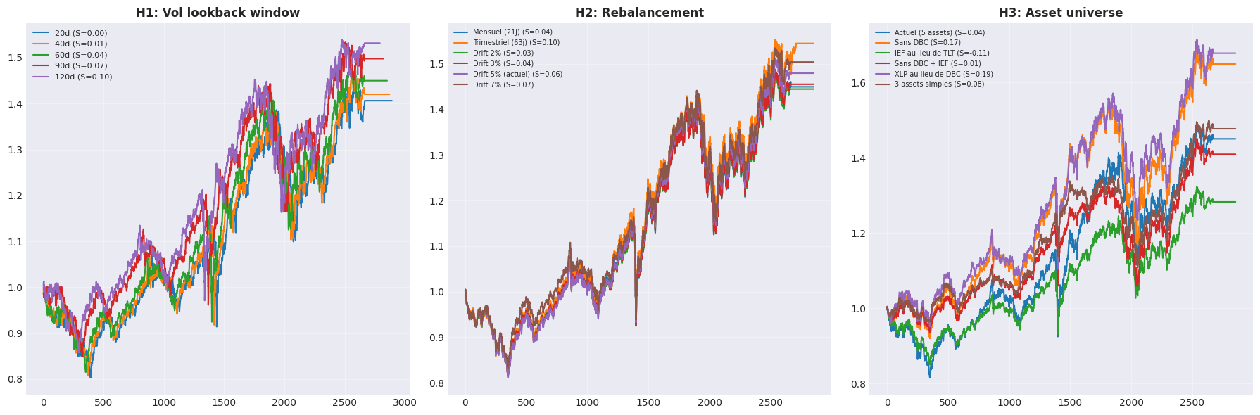
Vol Window        Sharpe     CAGR    MaxDD      Vol
--------------------------------------------------
20d                0.002    3.0%  -20.7%    8.8%
40d                0.014    3.1%  -20.2%    8.9%
60d                0.037    3.3%  -20.4%    9.0%
90d                0.074    3.7%  -20.0%    9.0%
120d               0.101    3.9%  -19.9%    9.1%
Verdict H1
60d est le standard. 20d trop reactif (bruit), 120d trop lent (retard).
4. Hypothese 2: Drift trigger vs rebal fixe
print (f" { 'Rebalancement' :<20} { 'Sharpe' :>8} { 'CAGR' :>8} { 'MaxDD' :>8} " )print ("-" * 45 )= {}for name, freq, drift in ['Mensuel (21j)' , 21 , None ),'Trimestriel (63j)' , 63 , None ),'Drift 2%' , 252 , 0.02 ),'Drift 3%' , 252 , 0.03 ),'Drift 5% (actuel)' , 252 , 0.05 ),'Drift 7%' , 252 , 0.07 ),= backtest_risk_parity(closes, base_assets, vol_window= 60 ,= freq, drift_trigger= drift)= rprint (f" { name:<20} { r['sharpe' ]:>8.3f} { r['cagr' ]:>7.1%} { r['max_dd' ]:>7.1%} " )
Rebalancement          Sharpe     CAGR    MaxDD
---------------------------------------------
Mensuel (21j)           0.037    3.3%  -20.4%
Trimestriel (63j)       0.101    3.9%  -19.9%
Drift 2%                0.034    3.3%  -19.9%
Drift 3%                0.042    3.4%  -19.8%
Drift 5% (actuel)       0.059    3.5%  -19.4%
Drift 7%                0.075    3.7%  -20.0%
Verdict H2
Règle #7 du backlog: Drift rebalancing > SMA overlay pour portfolios statiques. Verifier si drift 5% est optimal ou si 3% est meilleur.
5. Hypothese 3: Composition de l’univers
Tester différentes combinaisons d’actifs. DBC (contango structurel) et TLT (hausse des taux 2022) sont les candidats a remplacer.
= {'Actuel (5 assets)' : ['SPY' , 'EFA' , 'GLD' , 'DBC' , 'TLT' ],'Sans DBC' : ['SPY' , 'EFA' , 'GLD' , 'TLT' ],'IEF au lieu de TLT' : ['SPY' , 'EFA' , 'GLD' , 'DBC' , 'IEF' ],'Sans DBC + IEF' : ['SPY' , 'EFA' , 'GLD' , 'IEF' ],'XLP au lieu de DBC' : ['SPY' , 'EFA' , 'GLD' , 'XLP' , 'TLT' ],'3 assets simples' : ['SPY' , 'GLD' , 'IEF' ],print (f" { 'Univers' :<25} { 'Sharpe' :>8} { 'CAGR' :>8} { 'MaxDD' :>8} " )print ("-" * 50 )= {}for name, assets in universes.items():= [a for a in assets if a in closes.columns]= backtest_risk_parity(closes, avail, vol_window= 60 , rebal_freq= 21 )= rprint (f" { name:<25} { r['sharpe' ]:>8.3f} { r['cagr' ]:>7.1%} { r['max_dd' ]:>7.1%} " )
Univers                     Sharpe     CAGR    MaxDD
--------------------------------------------------
Actuel (5 assets)            0.037    3.3%  -20.4%
Sans DBC                     0.168    4.5%  -24.8%
IEF au lieu de TLT          -0.109    2.2%  -17.5%
Sans DBC + IEF               0.010    3.1%  -20.1%
XLP au lieu de DBC           0.185    4.7%  -21.5%
3 assets simples             0.080    3.5%  -18.0%
Verdict H3
Règle #3: TLT risk-off detruit la valeur. DBC = contango structurel. Verifier si des univers simplifies performent mieux.
6. Visualisation
= plt.subplots(1 , 3 , figsize= (18 , 6 ))# H1: Vol window = axes[0 ]for name, r in results_vol.items():'cum' ].values, label= f" { name} (S= { r['sharpe' ]:.2f} )" , linewidth= 1.5 )'H1: Vol lookback window' , fontweight= 'bold' )= 8 )True , alpha= 0.3 )# H2: Rebalancement = axes[1 ]for name, r in results_rebal.items():'cum' ].values, label= f" { name} (S= { r['sharpe' ]:.2f} )" , linewidth= 1.5 )'H2: Rebalancement' , fontweight= 'bold' )= 7 )True , alpha= 0.3 )# H3: Univers = axes[2 ]for name, r in results_univ.items():'cum' ].values, label= f" { name} (S= { r['sharpe' ]:.2f} )" , linewidth= 1.5 )'H3: Asset universe' , fontweight= 'bold' )= 7 )True , alpha= 0.3 )'riskparity_quantbook_analysis.png' , dpi= 150 , bbox_inches= 'tight' )
7. Conclusions
Tableau recapitulatif
H1 Vol window
(a remplir)
(a verifier)
H2 Rebalancement
(a remplir)
(a verifier)
H3 Univers
(a remplir)
(a verifier)
Règles du backlog appliquees
Règle #3: TLT risk-off detruit la valeur
Règle #7: Drift rebalancing > SMA overlay
Règle #9: Vol window 60d > 20d
Règle #17: Divergence yfinance documentee