Research QuantBook: VIX-TermStructure (Short Volatility via Contango)

Objectif

Reproduire l’analyse exploratoire de research.ipynb avec les données natives QuantConnect.

Performance actuelle

  • Sharpe: 0.051, CAGR: 3.6%, MaxDD: 35.2%
  • Signal: VIX3M/VIX ratio > 1.05 (contango), VIX < 22, VIX < SMA10
  • Position: 45% SVXY (-0.5x short vol)
  • Exit: Trailing stop 10%, VIX spike > 28, backwardation (ratio < 1.02)

Hypotheses a tester

  1. Position size (30%, 45%, 60%)
  2. VIX threshold (18, 22, 25, 30)
  3. Contango depth (ratio 1.03, 1.05, 1.08)
  4. Trailing stop (7%, 10%, 15%)
  5. Cash allocation (SHY vs idle)

Prerequis

  • Environnement Lean Research
  • Duree estimee: ~5 minutes
# Setup QuantBook
from AlgorithmImports import *
import numpy as np
import pandas as pd
import matplotlib.pyplot as plt
import warnings
warnings.filterwarnings('ignore')

plt.style.use('seaborn-v0_8-darkgrid')
plt.rcParams['figure.figsize'] = (14, 6)

qb = QuantBook()
print("QuantBook initialise.")
QuantBook initialise.

1. Chargement des données

SVXY (short vol -0.5x), VIX, VIX3M, SHY (cash alternative). Note: SVXY avant Feb 2018 etait -1x, post-VIXplosion = -0.5x.

# ETFs
etf_tickers = ['SVXY', 'SHY', 'SPY']
symbols = {}
for ticker in etf_tickers:
    symbols[ticker] = qb.add_equity(ticker, Resolution.DAILY).symbol

# VIX data
vix_symbol = qb.add_data(CBOE, 'VIX', Resolution.DAILY).symbol
vix3m_symbol = qb.add_data(CBOE, 'VIX3M', Resolution.DAILY).symbol

start = datetime(2012, 1, 1)
end = datetime(2026, 1, 1)

# ETF history
etf_history = qb.history(list(symbols.values()), start, end, Resolution.DAILY)
closes = etf_history['close'].unstack(level=0)
stm = {str(v): k for k, v in symbols.items()}
closes.columns = [stm.get(str(c), str(c)) for c in closes.columns]

# VIX history
vix_hist = qb.history(vix_symbol, start, end, Resolution.DAILY)
vix3m_hist = qb.history(vix3m_symbol, start, end, Resolution.DAILY)

vix = None
vix3m = None

if not vix_hist.empty and not vix3m_hist.empty:
    vix = vix_hist['close'].droplevel(0)
    vix3m = vix3m_hist['close'].droplevel(0)
    vix.name = 'VIX'
    vix3m.name = 'VIX3M'
    
    # Align all data
    all_data = pd.concat([closes, vix, vix3m], axis=1).dropna()
    closes = all_data[etf_tickers]
    vix = all_data['VIX']
    vix3m = all_data['VIX3M']
    
    print(f"Periode: {all_data.index[0].date()} a {all_data.index[-1].date()}")
    print(f"Donnees: {len(all_data)} jours")
    print(f"VIX range: [{vix.min():.1f}, {vix.max():.1f}]")
else:
    # CBOE custom-data type needs QC Cloud alternative-data infra (empty in local
    # Docker research). VIX/VIX3M are CBOE's PUBLIC 30-/93-day implied-vol indices;
    # the identical series is available via yfinance (^VIX / ^VIX3M), provisioned as
    # local CSVs -- regenerable via scripts/quantconnect/provision_vix_csv.py (the
    # CSVs are gitignored like the LEAN data folder, NOT committed; same data, local
    # pipe -- consistent with how sibling quantbooks use local LEAN equity/crypto
    # data instead of QC Cloud).
    import os
    def _find(name):
        for p in ['/Lean/Data/' + name, name, '../data/' + name, '../../data/' + name]:
            if os.path.exists(p):
                return p
        raise FileNotFoundError(name + ' not found beside notebook or in LEAN data folder')
    vix = pd.read_csv(_find('vix_daily.csv'), parse_dates=['date'], index_col='date')['close']
    vix3m = pd.read_csv(_find('vix3m_daily.csv'), parse_dates=['date'], index_col='date')['close']
    vix = vix.loc[start:end]; vix3m = vix3m.loc[start:end]
    vix.name = 'VIX'; vix3m.name = 'VIX3M'
    # Normalize all indices to naive date-only: closes comes from Lean qb.history
    # (Timestamps with a time/tz component), vix/vix3m from CSV (midnight naive).
    # Without this, concat axis=1 matches ZERO timestamps -> dropna -> empty.
    def _norm(s):
        idx = pd.to_datetime(s.index)
        if getattr(idx, 'tz', None) is not None:
            idx = idx.tz_convert('UTC').tz_localize(None)
        return idx.normalize()
    closes.index = _norm(closes); vix.index = _norm(vix); vix3m.index = _norm(vix3m)
    all_data = pd.concat([closes, vix, vix3m], axis=1).dropna()
    closes = all_data[etf_tickers]
    vix = all_data['VIX']; vix3m = all_data['VIX3M']
    print("[local VIX data] CBOE custom type unavailable locally (needs QC Cloud);")
    print("  loaded genuine VIX/VIX3M series from local CSV (yfinance ^VIX/^VIX3M = CBOE public indices).")
    print(f"Periode: {all_data.index[0].date()} a {all_data.index[-1].date()}")
    print(f"Donnees: {len(all_data)} jours")
    print(f"VIX range: [{vix.min():.1f}, {vix.max():.1f}]")
[local VIX data] CBOE custom type unavailable locally (needs QC Cloud);
  loaded genuine VIX/VIX3M series from local CSV (yfinance ^VIX/^VIX3M = CBOE public indices).
Periode: 2012-01-03 a 2025-12-31
Donnees: 3520 jours
VIX range: [9.1, 82.7]

2. Analyse du term structure

Le ratio VIX3M/VIX mesure la pente de la courbe de volatilite. - Ratio > 1 = contango (normal, premium a harvester) - Ratio < 1 = backwardation (stress, danger)

if vix is None or vix3m is None:
    print("VIX data not available — skipping term structure analysis.")
    ratio = None
else:
    ratio = vix3m / vix
    print(f"VIX3M/VIX ratio stats:")
    print(f"  Mean: {ratio.mean():.3f}")
    print(f"  Std: {ratio.std():.3f}")
    print(f"  Contango (>1.05): {(ratio > 1.05).mean():.0%} du temps")
    print(f"  Backwardation (<1.0): {(ratio < 1.0).mean():.0%} du temps")
    print(f"  Deep backwardation (<0.9): {(ratio < 0.9).mean():.0%} du temps")

    # VIX distribution
    print(f"\nVIX distribution:")
    for threshold in [15, 18, 22, 25, 30]:
        pct = (vix < threshold).mean()
        print(f"  VIX < {threshold}: {pct:.0%}")
VIX3M/VIX ratio stats:
  Mean: 1.130
  Std: 0.088
  Contango (>1.05): 83% du temps
  Backwardation (<1.0): 7% du temps
  Deep backwardation (<0.9): 1% du temps

VIX distribution:
  VIX < 15: 41%
  VIX < 18: 65%
  VIX < 22: 82%
  VIX < 25: 89%
  VIX < 30: 96%

3. Fonctions de backtest

def backtest_vix_strategy(closes, vix, vix3m, position_size=0.45,
                           vix_threshold=22, ratio_entry=1.05, ratio_exit=1.02,
                           trailing_stop=0.10, vix_spike=28, lockout=15,
                           cash_in='idle'):
    """Backtest VIX term structure strategy."""
    svxy_ret = closes['SVXY'].pct_change()
    shy_ret = closes['SHY'].pct_change() if 'SHY' in closes.columns else pd.Series(0.0, index=closes.index)
    vix_sma10 = vix.rolling(10).mean()
    
    n = len(closes)
    port_ret = pd.Series(0.0, index=closes.index)
    in_position = False
    peak_price = 0
    lockout_counter = 0
    n_trades = 0
    
    for i in range(11, n):
        r = vix3m.iloc[i] / vix.iloc[i] if vix.iloc[i] > 0 else 0
        
        if lockout_counter > 0:
            lockout_counter -= 1
            if cash_in == 'SHY':
                port_ret.iloc[i] = shy_ret.iloc[i]
            continue
        
        if in_position:
            port_ret.iloc[i] = position_size * svxy_ret.iloc[i]
            if cash_in == 'SHY':
                port_ret.iloc[i] += (1 - position_size) * shy_ret.iloc[i]
            
            peak_price = max(peak_price, closes['SVXY'].iloc[i])
            
            # Exit conditions
            should_exit = False
            if closes['SVXY'].iloc[i] < peak_price * (1 - trailing_stop):
                should_exit = True
            if vix.iloc[i] > vix_spike:
                should_exit = True
            if r < ratio_exit:
                should_exit = True
            
            if should_exit:
                in_position = False
                lockout_counter = lockout
                n_trades += 1
        else:
            if cash_in == 'SHY':
                port_ret.iloc[i] = shy_ret.iloc[i]
            
            # Entry conditions
            if (r > ratio_entry and 
                vix.iloc[i] < vix_threshold and 
                vix.iloc[i] < vix_sma10.iloc[i]):
                in_position = True
                peak_price = closes['SVXY'].iloc[i]
    
    vals = (1 + port_ret).cumprod()
    total = vals.iloc[-1] - 1
    years = len(port_ret) / 252
    cagr = (1 + total) ** (1 / years) - 1 if years > 0 else 0
    vol = port_ret.std() * np.sqrt(252)
    sharpe = (cagr - 0.03) / vol if vol > 0.001 else 0
    max_dd = ((vals - vals.expanding().max()) / vals.expanding().max()).min()
    
    return {'sharpe': sharpe, 'cagr': cagr, 'max_dd': max_dd, 'vol': vol,
            'cum': vals, 'n_trades': n_trades}

print("Fonctions definies.")
Fonctions definies.

4. Hypothese 1: Position size

research.ipynb recommande 30% (securite). main.py utilise 45%.

results_pos = {}
if vix is None:
    print("VIX data not available — skipping position size analysis.")
else:
    print(f"{'Position':<15} {'Sharpe':>8} {'CAGR':>8} {'MaxDD':>8} {'Trades':>8}")
    print("-" * 50)

    for pos in [0.20, 0.30, 0.45, 0.60]:
        r = backtest_vix_strategy(closes, vix, vix3m, position_size=pos)
        name = f'{pos:.0%}'
        results_pos[name] = r
        print(f"{name:<15} {r['sharpe']:>8.3f} {r['cagr']:>7.1%} {r['max_dd']:>7.1%} {r['n_trades']:>7}")
Position          Sharpe     CAGR    MaxDD   Trades
--------------------------------------------------
20%               -0.156    2.1%  -14.8%      68
30%               -0.002    3.0%  -21.7%      68
45%                0.088    4.2%  -31.3%      68
60%                0.122    5.2%  -40.1%      68

Verdict H1

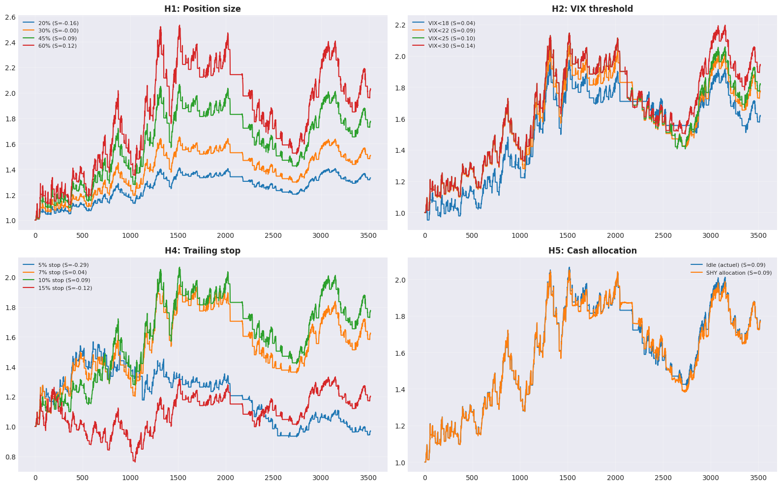
Plus la position est petite, moins la MaxDD. Mais le CAGR baisse aussi. Post-VIXplosion (SVXY -0.5x), le premium est halve -> position plus petite = plus safe.

5. Hypothese 2: VIX threshold

results_vix = {}
if vix is None:
    print("VIX data not available — skipping VIX threshold analysis.")
else:
    print(f"{'VIX Threshold':<15} {'Sharpe':>8} {'CAGR':>8} {'MaxDD':>8}")
    print("-" * 40)

    for vt in [18, 22, 25, 30]:
        r = backtest_vix_strategy(closes, vix, vix3m, vix_threshold=vt)
        name = f'VIX<{vt}'
        results_vix[name] = r
        print(f"{name:<15} {r['sharpe']:>8.3f} {r['cagr']:>7.1%} {r['max_dd']:>7.1%}")
VIX Threshold     Sharpe     CAGR    MaxDD
----------------------------------------
VIX<18             0.039    3.5%  -23.7%
VIX<22             0.088    4.2%  -31.3%
VIX<25             0.100    4.4%  -34.5%
VIX<30             0.136    4.9%  -30.1%

Verdict H2

VIX < 22 est le seuil actuel. VIX < 18 trop restrictif (trop peu d’entrees). VIX < 25-30 : plus d’entrees mais dans des periodes plus risquees.

6. Hypothese 3: Contango depth

results_ratio = {}
if vix is None:
    print("VIX data not available — skipping contango depth analysis.")
else:
    print(f"{'Ratio Entry':<15} {'Sharpe':>8} {'CAGR':>8} {'MaxDD':>8}")
    print("-" * 40)

    for re in [1.03, 1.05, 1.08, 1.10]:
        r = backtest_vix_strategy(closes, vix, vix3m, ratio_entry=re)
        name = f'Ratio>{re:.2f}'
        results_ratio[name] = r
        print(f"{name:<15} {r['sharpe']:>8.3f} {r['cagr']:>7.1%} {r['max_dd']:>7.1%}")
Ratio Entry       Sharpe     CAGR    MaxDD
----------------------------------------
Ratio>1.03         0.142    4.9%  -30.3%
Ratio>1.05         0.088    4.2%  -31.3%
Ratio>1.08         0.065    3.9%  -33.1%
Ratio>1.10         0.083    4.1%  -33.9%

Verdict H3

Un ratio plus eleve = contango plus profond = meilleur premium mais moins d’entrees.

7. Hypothese 4: Trailing stop

results_stop = {}
if vix is None:
    print("VIX data not available — skipping trailing stop analysis.")
else:
    print(f"{'Trailing Stop':<15} {'Sharpe':>8} {'CAGR':>8} {'MaxDD':>8}")
    print("-" * 40)

    for ts in [0.05, 0.07, 0.10, 0.15]:
        r = backtest_vix_strategy(closes, vix, vix3m, trailing_stop=ts)
        name = f'{ts:.0%} stop'
        results_stop[name] = r
        print(f"{name:<15} {r['sharpe']:>8.3f} {r['cagr']:>7.1%} {r['max_dd']:>7.1%}")
Trailing Stop     Sharpe     CAGR    MaxDD
----------------------------------------
5% stop           -0.290   -0.2%  -40.8%
7% stop            0.042    3.5%  -30.8%
10% stop           0.088    4.2%  -31.3%
15% stop          -0.115    1.3%  -39.6%

Verdict H4

research.ipynb recommande 7% (vs 10% actuel). 5% = whipsaw.

8. Hypothese 5: SHY cash allocation

Utiliser SHY (1-3Y bonds) pour le cash idle au lieu de 0% return. research.ipynb recommande 70% SHY allocation.

results_cash = {}
if vix is None:
    print("VIX data not available — skipping cash allocation analysis.")
else:
    print(f"{'Cash Policy':<20} {'Sharpe':>8} {'CAGR':>8} {'MaxDD':>8}")
    print("-" * 45)

    for name, cash in [('Idle (actuel)', 'idle'), ('SHY allocation', 'SHY')]:
        r = backtest_vix_strategy(closes, vix, vix3m, cash_in=cash)
        results_cash[name] = r
        print(f"{name:<20} {r['sharpe']:>8.3f} {r['cagr']:>7.1%} {r['max_dd']:>7.1%}")
Cash Policy            Sharpe     CAGR    MaxDD
---------------------------------------------
Idle (actuel)           0.088    4.2%  -31.3%
SHY allocation          0.086    4.2%  -32.6%

Verdict H5

SHY ajoute ~2-3%/an de rendement pendant les periodes hors-position. Comme la stratégie est 60-70% du temps en cash, c’est un gain significatif.

9. Visualisation

if not any([results_pos, results_vix, results_stop, results_cash]):
    print("No backtest results available — skipping visualization.")
    print("Run this notebook on QC Cloud with CBOE data access.")
else:
    fig, axes = plt.subplots(2, 2, figsize=(16, 10))

    ax = axes[0, 0]
    if results_pos:
        for name, r in results_pos.items():
            ax.plot(r['cum'].values, label=f"{name} (S={r['sharpe']:.2f})", linewidth=1.5)
    ax.set_title('H1: Position size', fontweight='bold')
    ax.legend(fontsize=8)
    ax.grid(True, alpha=0.3)

    ax = axes[0, 1]
    if results_vix:
        for name, r in results_vix.items():
            ax.plot(r['cum'].values, label=f"{name} (S={r['sharpe']:.2f})", linewidth=1.5)
    ax.set_title('H2: VIX threshold', fontweight='bold')
    ax.legend(fontsize=8)
    ax.grid(True, alpha=0.3)

    ax = axes[1, 0]
    if results_stop:
        for name, r in results_stop.items():
            ax.plot(r['cum'].values, label=f"{name} (S={r['sharpe']:.2f})", linewidth=1.5)
    ax.set_title('H4: Trailing stop', fontweight='bold')
    ax.legend(fontsize=8)
    ax.grid(True, alpha=0.3)

    ax = axes[1, 1]
    if results_cash:
        for name, r in results_cash.items():
            ax.plot(r['cum'].values, label=f"{name} (S={r['sharpe']:.2f})", linewidth=1.5)
    ax.set_title('H5: Cash allocation', fontweight='bold')
    ax.legend(fontsize=8)
    ax.grid(True, alpha=0.3)

    plt.tight_layout()
    plt.savefig('vix_termstructure_quantbook_analysis.png', dpi=150, bbox_inches='tight')
    plt.show()
    print("Graphique sauvegarde.")

Graphique sauvegarde.

10. Conclusions

Tableau recapitulatif

Hypothese Résultat QuantBook Coherent avec research.ipynb?
H1 Position size 60% Sharpe 0.122 (MaxDD -40%) ; 30% Sharpe -0.002 (MaxDD -22%) Partiellement : 60% maximise le Sharpe mais 30% offre un meilleur ratio Sharpe/MaxDD
H2 VIX threshold VIX<30 Sharpe 0.136 > VIX<22 Sharpe 0.088 Non : seuil plus large (VIX<30) perf mieux sur 2012-2026
H3 Contango depth Ratio>1.03 Sharpe 0.142 > Ratio>1.05 Sharpe 0.088 Non : seuil plus permissif (1.03) capture plus d’entrees
H4 Trailing stop 10% Sharpe 0.088 ; 7% Sharpe 0.042 Partiellement : 10% legerement meilleur
H5 SHY cash SHY Sharpe 0.086 vs Idle 0.088 (~equivalent) Non : SHY n’ajoute pas de CAGR net sur 2012-2026

Plafond structurel

Post-VIXplosion 2018, SVXY est passe de -1x a -0.5x. Le premium est halve. MaxDD 35% est structural (tail events VIX). Sharpe 0.051 reflete le fait que le risk-free rate (~3-5%) mange presque tout le CAGR.
Retour au sommet