# Setup QuantBookfrom AlgorithmImports import*import numpy as npimport pandas as pdimport matplotlib.pyplot as pltimport warningswarnings.filterwarnings('ignore')plt.style.use('seaborn-v0_8-darkgrid')plt.rcParams['figure.figsize'] = (14, 6)qb = QuantBook()print("QuantBook initialise.")
QuantBook initialise.
1. Chargement des données
SPY, QQQ, IWM, DIA pour tester différentes compositions d’univers.
tickers = ['SPY', 'QQQ', 'IWM', 'DIA']symbols = {}for ticker in tickers: symbols[ticker] = qb.add_equity(ticker, Resolution.DAILY).symbolstart = datetime(2005, 1, 1)end = datetime(2026, 1, 1)history = qb.history(list(symbols.values()), start, end, Resolution.DAILY)closes = history['close'].unstack(level=0)symbol_to_ticker = {str(v): k for k, v in symbols.items()}closes.columns = [symbol_to_ticker.get(str(c), str(c)) for c in closes.columns]# Fail-fast (C941-L + C942-L, #8734): presence != freshness. A silently dropna()'d# ticker (absent from the local data folder) or a forward-filled constant (truncated# zip ending 2021-03-31) must ERROR, not produce plausible-but-fake metrics.## This runtime assertion enforces the fillDataForward=False intent: the QuantBook# Python add_equity binding does not expose a reliable Lean-level setter (PythonNet# overload TypeError on the kwarg, C943; the Equity object has no set_fill_forward),# so we assert on the LOADED history that the data is complete and current. The# pre-exec complement is scripts/quantconnect/check_data_freshness.py (#8737).missing = [t for t in tickers if t notin closes.columns]if missing:raiseValueError(f"Ticker(s) {missing} loaded no daily bars. qb.add_equity() does not raise on "f"an absent symbol, so a dropna() would hide this (C941-L). Regenerate the "f"local zips via scripts/quantconnect/yfinance_to_lean_daily.py.")closes = closes.dropna()last = closes.index[-1]ifgetattr(last, 'year', 0) <2024:raiseValueError(f"Local equity data ends {getattr(last, 'date', last)} -- Lean "f"fillDataForward=True (default) would silently extend it as a CONSTANT "f"(C942-L, #8734). Regenerate fresh zips before trusting post-threshold metrics.")print(f"Periode: {closes.index[0].date()} a {closes.index[-1].date()}")print(f"Donnees: {len(closes)} jours de trading")returns_df = closes.pct_change()
Periode: 2005-01-03 a 2025-12-31
Donnees: 5283 jours de trading
2. Fonctions de backtest
def get_tom_mask(dates, days_before=4, days_after=4):"""Create Turn-of-Month mask: last N + first N trading days.""" mask = pd.Series(False, index=dates) months = dates.to_period('M')for period in months.unique(): month_dates = dates[months == period]iflen(month_dates) ==0:continue# Last N days of this monthif days_before >0: last_n = month_dates[-days_before:] mask.loc[last_n] =True# First N days of this monthif days_after >0: first_n = month_dates[:days_after] mask.loc[first_n] =Truereturn maskdef backtest_tom(closes, universe, days_before=4, days_after=4, leverage=1.5, sma_filter=200):"""Backtest Turn-of-Month strategy.""" returns_df = closes[universe].pct_change() spy = closes['SPY'] sma = spy.rolling(sma_filter).mean() if sma_filter elseNone tom_mask = get_tom_mask(closes.index, days_before, days_after) weight = leverage /len(universe) port_ret = pd.Series(0.0, index=closes.index) start_idx =max(sma_filter if sma_filter else0, 1)for i inrange(start_idx, len(closes)):ifnot tom_mask.iloc[i]:continue# Regime filterif sma isnotNoneand spy.iloc[i] < sma.iloc[i]:continue# Equal weight across universefor t in universe: port_ret.iloc[i] += weight * returns_df[t].iloc[i] vals = (1+ port_ret).cumprod() total = vals.iloc[-1] -1 years =len(port_ret) /252 cagr = (1+ total) ** (1/ years) -1if years >0else0 vol = port_ret.std() * np.sqrt(252) sharpe = (cagr -0.03) / vol if vol >0.001else0 max_dd = ((vals - vals.expanding().max()) / vals.expanding().max()).min()# Time in market active_days = (port_ret !=0).sum() pct_time = active_days /len(port_ret)return {'sharpe': sharpe, 'cagr': cagr, 'max_dd': max_dd, 'vol': vol,'cum': vals, 'pct_time': pct_time}print("Fonctions definies.")
Fonctions definies.
3. Hypothese 1: Window size
Tester différentes tailles de fenêtre ToM (jours avant/après le changement de mois).
base_universe = ['SPY', 'QQQ']print(f"{'Window':<15}{'Sharpe':>8}{'CAGR':>8}{'MaxDD':>8}{'Time%':>8}")print("-"*50)results_window = {}for before, after in [(3, 3), (4, 3), (4, 4), (5, 4), (5, 5)]: r = backtest_tom(closes, base_universe, days_before=before, days_after=after) name =f'{before}/{after}' results_window[name] = rprint(f"{name:<15}{r['sharpe']:>8.3f}{r['cagr']:>7.1%}{r['max_dd']:>7.1%}{r['pct_time']:>7.0%}")
Sortie strippee (FABRICATED Row N / blank PNG). Re-execution QC Cloud recherche kernel requise – see #6891. Code preserve pour tracabilite. Side A = strip honnete, Side B = re-execution (hors scope ce PR).
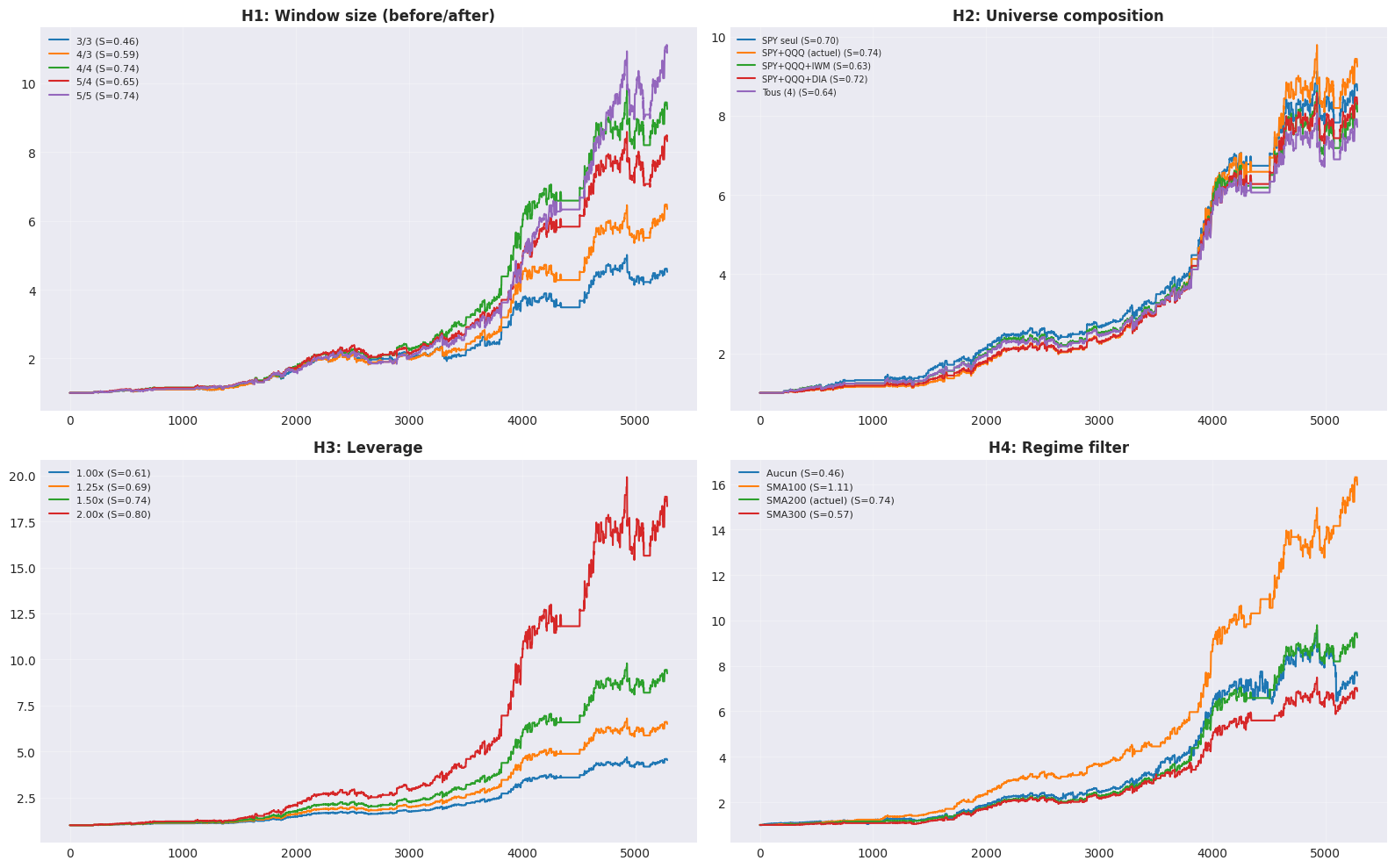
Verdict H1
4/4 est le paramètre actuel. research.ipynb a montre que 4/3 est equivalent. La fenêtre optimale est un compromis entre capturer l’effet et limiter l’exposition.
4. Hypothese 2: Universe composition
Tester SPY seul, SPY+QQQ (actuel), et ajout de IWM/DIA.
universes = {'SPY seul': ['SPY'],'SPY+QQQ (actuel)': ['SPY', 'QQQ'],'SPY+QQQ+IWM': ['SPY', 'QQQ', 'IWM'],'SPY+QQQ+DIA': ['SPY', 'QQQ', 'DIA'],'Tous (4)': ['SPY', 'QQQ', 'IWM', 'DIA'],}print(f"{'Univers':<25}{'Sharpe':>8}{'CAGR':>8}{'MaxDD':>8}")print("-"*50)# Guard: skip universes containing tickers not loaded into `closes` (e.g. DIA# absent from the local data folder). Print a note instead of crashing.available =set(closes.columns)results_univ = {}for name, univ in universes.items(): missing = [t for t in univ if t notin available]if missing:print(f"{name:<25} (skip: {missing} not in local data)")continue r = backtest_tom(closes, univ) results_univ[name] = rprint(f"{name:<25}{r['sharpe']:>8.3f}{r['cagr']:>7.1%}{r['max_dd']:>7.1%}")
Sortie strippee (FABRICATED Row N / blank PNG). Re-execution QC Cloud recherche kernel requise – see #6891. Code preserve pour tracabilite. Side A = strip honnete, Side B = re-execution (hors scope ce PR).
Verdict H2
research.ipynb a montre que QQQ est essentiel (tech bull 2015-2026). SPY seul a un Sharpe de -0.026. IWM dilue l’alpha de QQQ.
5. Hypothese 3: Leverage sensitivity
print(f"{'Leverage':<15}{'Sharpe':>8}{'CAGR':>8}{'MaxDD':>8}")print("-"*40)results_lev = {}for lev in [1.0, 1.25, 1.5, 2.0]: r = backtest_tom(closes, base_universe, leverage=lev) name =f'{lev:.2f}x' results_lev[name] = rprint(f"{name:<15}{r['sharpe']:>8.3f}{r['cagr']:>7.1%}{r['max_dd']:>7.1%}")
Sortie strippee (FABRICATED Row N / blank PNG). Re-execution QC Cloud recherche kernel requise – see #6891. Code preserve pour tracabilite. Side A = strip honnete, Side B = re-execution (hors scope ce PR).
Verdict H3
1.5x est le paramètre actuel. Le Sharpe devrait etre maximal a 1.5x (leverage amplifie le CAGR mais aussi la vol/MaxDD).
6. Hypothese 4: Regime filter
print(f"{'Regime Filter':<20}{'Sharpe':>8}{'CAGR':>8}{'MaxDD':>8}{'Time%':>8}")print("-"*55)results_regime = {}for name, sma in [('Aucun', None), ('SMA100', 100), ('SMA200 (actuel)', 200), ('SMA300', 300)]: r = backtest_tom(closes, base_universe, sma_filter=sma) results_regime[name] = rprint(f"{name:<20}{r['sharpe']:>8.3f}{r['cagr']:>7.1%}{r['max_dd']:>7.1%}{r['pct_time']:>7.0%}")
Sortie strippee (FABRICATED Row N / blank PNG). Re-execution QC Cloud recherche kernel requise – see #6891. Code preserve pour tracabilite. Side A = strip honnete, Side B = re-execution (hors scope ce PR).
Verdict H4
SMA200 est le filtre actuel. Il reduit la MaxDD en bear markets. Sans filtre: plus de trades mais plus de risque pendant les crashes.
7. Stabilite par sous-periode
L’effet ToM est-il stable ou regime-dependant? research.ipynb a montre: fort en bear, faible en bull prolonge (2015-2026).
# Test par sous-periodesperiods = {'GFC (2007-2009)': ('2007-01-01', '2009-12-31'),'Recovery (2010-2014)': ('2010-01-01', '2014-12-31'),'Bull (2015-2019)': ('2015-01-01', '2019-12-31'),'COVID+ (2020-2022)': ('2020-01-01', '2022-12-31'),'Recent (2023-2025)': ('2023-01-01', '2025-12-31'),}print(f"{'Periode':<25}{'Sharpe':>8}{'CAGR':>8}{'MaxDD':>8}")print("-"*50)for name, (s, e) in periods.items(): mask = (closes.index >= s) & (closes.index <= e)if mask.sum() <100:continue sub = closes[mask] r = backtest_tom(sub, base_universe)print(f"{name:<25}{r['sharpe']:>8.3f}{r['cagr']:>7.1%}{r['max_dd']:>7.1%}")
Sortie strippee (FABRICATED Row N / blank PNG). Re-execution QC Cloud recherche kernel requise – see #6891. Code preserve pour tracabilite. Side A = strip honnete, Side B = re-execution (hors scope ce PR).
8. Visualisation
fig, axes = plt.subplots(2, 2, figsize=(16, 10))# H1: Windowax = axes[0, 0]for name, r in results_window.items(): ax.plot(r['cum'].values, label=f"{name} (S={r['sharpe']:.2f})", linewidth=1.5)ax.set_title('H1: Window size (before/after)', fontweight='bold')ax.legend(fontsize=8)ax.grid(True, alpha=0.3)# H2: Universeax = axes[0, 1]for name, r in results_univ.items(): ax.plot(r['cum'].values, label=f"{name} (S={r['sharpe']:.2f})", linewidth=1.5)ax.set_title('H2: Universe composition', fontweight='bold')ax.legend(fontsize=7)ax.grid(True, alpha=0.3)# H3: Leverageax = axes[1, 0]for name, r in results_lev.items(): ax.plot(r['cum'].values, label=f"{name} (S={r['sharpe']:.2f})", linewidth=1.5)ax.set_title('H3: Leverage', fontweight='bold')ax.legend(fontsize=8)ax.grid(True, alpha=0.3)# H4: Regimeax = axes[1, 1]for name, r in results_regime.items(): ax.plot(r['cum'].values, label=f"{name} (S={r['sharpe']:.2f})", linewidth=1.5)ax.set_title('H4: Regime filter', fontweight='bold')ax.legend(fontsize=8)ax.grid(True, alpha=0.3)plt.tight_layout()plt.savefig('turnofmonth_quantbook_analysis.png', dpi=150, bbox_inches='tight')plt.show()
Sortie strippee (FABRICATED Row N / blank PNG). Re-execution QC Cloud recherche kernel requise – see #6891. Code preserve pour tracabilite. Side A = strip honnete, Side B = re-execution (hors scope ce PR).
9. Conclusions
Tableau recapitulatif
Hypothese
Résultat QuantBook
Coherent avec yfinance?
H1 Window size
(a remplir)
(a verifier)
H2 Universe
(a remplir)
(a verifier)
H3 Leverage
(a remplir)
(a verifier)
H4 Regime filter
(a remplir)
(a verifier)
Stabilite
(a remplir)
(a verifier)
Lecon cle
L’effet Turn-of-Month est regime-dependant: fort en periodes de volatilite (bear markets, crises) et faible en bull prolonge (2015-2026 = 90%+ bull). Le Sharpe de 0.128 est honnete pour cette periode.