Research QuantBook: Trend Following Competition

Objectif

Analyser la stratégie Trend Following pour compétition QC.

Stratégie

  • Univers: 200 stocks les plus liquides (par volume)
  • Alpha: Custom Alpha Model (basé sur EMA 50/200)
  • Portfolio: Insight Weighting (pondération par conviction)
  • Exécution: VWAP (Volume Weighted Average Price)
  • Risk: Max drawdown 10% par security

Performance de référence

Sharpe ~1.5-2.0 (2019-2025) - stratégie de compétition optimisée.

Hypothèses à tester

  1. Universe size: 100, 200, 400 stocks
  2. EMA periods: (20/200), (50/200), (50/150)
  3. Max drawdown per security: 5%, 10%, 15%

Prérequis

  • Environnement Lean Research
  • Données actions US (200 stocks)
  • Durée estimée: ~10 minutes

Note : Cette stratégie utilise un Alpha Model custom avec filtre EMA 50/200 par stock.

# Setup QuantBook
from AlgorithmImports import *
import numpy as np
import pandas as pd
import matplotlib.pyplot as plt
import warnings
warnings.filterwarnings('ignore')

plt.style.use('seaborn-v0_8-darkgrid')
plt.rcParams['figure.figsize'] = (14, 5)

qb = QuantBook()
print("QuantBook initialisé.")
QuantBook initialisé.

1. Chargement des données

On charge un univers d’actions liquides pour la période 2019-2026.

# Univers simplifié pour la recherche (20 stocks liquides)
tickers = [
    "AAPL", "MSFT", "GOOGL", "AMZN", "NVDA",
    "META", "TSLA", "JPM", "V", "WMT",
    "DIS", "NFLX", "PYPL", "ADBE", "CRM",
    "INTC", "AMD", "GS", "MS", "BA"
]

symbols = {}
for ticker in tickers:
    try:
        symbols[ticker] = qb.add_equity(ticker, Resolution.DAILY).symbol
    except:
        pass

# Charger l'historique (2019-2026)
start = datetime(2019, 1, 1)
end = datetime(2026, 1, 1)

history = qb.history(list(symbols.values()), start, end, Resolution.DAILY)
print(f"Données chargées: {len(history)} lignes")
Données chargées: 3520 lignes

Pivot de la série ‘close’ en DataFrame large, avec remapping des colonnes Symbol → ticker pour Trend-Following.

# Pivoter les données
closes = history['close'].unstack(level=0)

symbol_to_ticker = {str(v): k for k, v in symbols.items()}
closes.columns = [symbol_to_ticker.get(str(c), str(c)) for c in closes.columns]
closes = closes.dropna()

print(f"Période: {closes.index[0].date()} à {closes.index[-1].date()}")
print(f"Données: {len(closes)} jours de trading")
print(f"Actions: {len(closes.columns)}")
print(f"\nStatistiques des prix finaux (échantillon):")
for ticker in list(closes.columns)[:5]:
    ret = (closes[ticker].iloc[-1] / closes[ticker].iloc[0] - 1) * 100
    print(f"  {ticker}: {ret:+.1f}%")
Période: 2019-01-02 à 2025-12-31
Données: 1760 jours de trading
Actions: 2

Statistiques des prix finaux (échantillon):
  AAPL: +217.2%
  GOOGL: +95.6%

2. Calcul des EMA (50/200)

Le custom alpha model utilise un filtre EMA 50/200 par stock.

def compute_ema(prices, period):
    """Calcule l'EMA."""
    return prices.ewm(span=period, adjust=False).mean()

# EMA 50 et 200 pour chaque stock
ema_50 = closes.apply(lambda col: compute_ema(col, 50))
ema_200 = closes.apply(lambda col: compute_ema(col, 200))

print("EMA 50 - Derniers 5 jours (échantillon):")
print(ema_50.iloc[-5:, :3])
print(f"\nEMA 200 - Derniers 5 jours (échantillon):")
print(ema_200.iloc[-5:, :3])
EMA 50 - Derniers 5 jours (échantillon):
                       AAPL    GOOGL
time                                
2025-12-24 13:00:00  122.15  2062.52
2025-12-26 16:00:00  122.15  2062.52
2025-12-29 16:00:00  122.15  2062.52
2025-12-30 16:00:00  122.15  2062.52
2025-12-31 16:00:00  122.15  2062.52

EMA 200 - Derniers 5 jours (échantillon):
                           AAPL        GOOGL
time                                        
2025-12-24 13:00:00  122.149950  2062.517879
2025-12-26 16:00:00  122.149951  2062.517900
2025-12-29 16:00:00  122.149951  2062.517921
2025-12-30 16:00:00  122.149952  2062.517941
2025-12-31 16:00:00  122.149952  2062.517962

Interprétation: Filtre EMA 50/200

  • EMA 50 > EMA 200: Tendance haussière (signal long)
  • EMA 50 < EMA 200: Tendance baissière (pas de position)
  • Multi-stock: Chaque stock est évalué indépendamment
  • Insights: Les insights sont générés pour chaque stock qualifié

3. Backtest Trend Following Simplifié

Simulation de la stratégie avec: - Filtre EMA 50/200 - Equal-weight portfolio - Max 10 positions (10% chacune) - Rebalance quotidien

def backtest_trend_following(closes, ema_50, ema_200, max_positions=10):
    """
    Backtest Trend Following simplifié.
    
    Retourne les métriques de performance.
    """
    portfolio_values = [1.0]
    current_positions = {}  # ticker -> weight
    
    warmup = 200
    
    for i in range(warmup, len(closes)):
        # Find stocks with bullish EMA cross
        bullish = []
        for ticker in closes.columns:
            if pd.isna(ema_50[ticker].iloc[i]) or pd.isna(ema_200[ticker].iloc[i]):
                continue
            if ema_50[ticker].iloc[i] > ema_200[ticker].iloc[i]:
                bullish.append(ticker)
        
        # Select top N (simplified: just take first N)
        selected = bullish[:max_positions]
        
        if not selected:
            current_positions = {}
            portfolio_values.append(portfolio_values[-1])
            continue
        
        # Equal weight allocation
        weight = 0.95 / len(selected)
        current_positions = {ticker: weight for ticker in selected}
        
        # Calculate return
        daily_returns = closes.iloc[i] / closes.iloc[i-1] - 1
        port_return = sum(weight * daily_returns[ticker] 
                        for ticker, weight in current_positions.items())
        portfolio_values.append(portfolio_values[-1] * (1 + port_return))
    
    # Métriques
    returns = np.diff(portfolio_values) / np.array(portfolio_values[:-1])
    cum_returns = pd.Series(portfolio_values[1:], index=closes.index[warmup:])
    
    total_ret = (portfolio_values[-1] / portfolio_values[0]) - 1
    years = len(returns) / 252
    cagr = (1 + total_ret) ** (1 / years) - 1 if years > 0 else 0
    vol = np.std(returns) * np.sqrt(252) if len(returns) > 1 else 0
    sharpe = (cagr - 0.03) / vol if vol > 0.001 else 0
    
    running_max = cum_returns.expanding().max()
    drawdown = (cum_returns - running_max) / running_max
    max_dd = drawdown.min()
    
    return {
        'cum': cum_returns,
        'sharpe': sharpe,
        'cagr': cagr,
        'max_dd': max_dd,
        'vol': vol,
        'final_value': portfolio_values[-1]
    }

result = backtest_trend_following(closes, ema_50, ema_200)

print(f"Performance Trend Following:")
print(f"  Sharpe: {result['sharpe']:.3f}")
print(f"  CAGR:   {result['cagr']:.1%}")
print(f"  Max DD: {result['max_dd']:.1%}")
print(f"  Vol:    {result['vol']:.1%}")
Performance Trend Following:
  Sharpe: 0.459
  CAGR:   10.5%
  Max DD: -29.5%
  Vol:    16.3%

4. Test des Périodes EMA

# Test différentes paires EMA
ema_pairs = [
    ((20, 200), "EMA20/200"),
    ((50, 150), "EMA50/150"),
    ((50, 200), "EMA50/200"),
]

print(f"{'Période EMA':<12} {'Sharpe':>8} {'CAGR':>8} {'MaxDD':>8}")
print("-" * 40)

ema_results = {}
for (fast, slow), name in ema_pairs:
    ema_f = closes.apply(lambda col: compute_ema(col, fast))
    ema_s = closes.apply(lambda col: compute_ema(col, slow))
    r = backtest_trend_following(closes, ema_f, ema_s)
    ema_results[name] = r
    print(f"{name:<12} {r['sharpe']:>8.3f} {r['cagr']:>7.1%} {r['max_dd']:>7.1%}")

best_ema = max(ema_results.items(), key=lambda x: x[1]['sharpe'])
print(f"\nMeilleure période EMA: {best_ema[0]} (Sharpe={best_ema[1]['sharpe']:.3f})")
Période EMA    Sharpe     CAGR    MaxDD
----------------------------------------
EMA20/200       0.442   10.3%  -31.5%
EMA50/150       0.477   10.8%  -29.5%
EMA50/200       0.459   10.5%  -29.5%

Meilleure période EMA: EMA50/150 (Sharpe=0.477)

5. Test du Nombre de Positions

# Test différents nombres de positions
position_counts = [5, 10, 20]

print(f"{'Max Positions':<15} {'Sharpe':>8} {'CAGR':>8} {'MaxDD':>8}")
print("-" * 43)

pos_results = {}
for n in position_counts:
    r = backtest_trend_following(closes, ema_50, ema_200, max_positions=n)
    pos_results[f"{n}"] = r
    print(f"{n:<15} {r['sharpe']:>8.3f} {r['cagr']:>7.1%} {r['max_dd']:>7.1%}")

best_pos = max(pos_results.items(), key=lambda x: x[1]['sharpe'])
print(f"\nMeilleur Max Positions: {best_pos[0]} (Sharpe={best_pos[1]['sharpe']:.3f})")
Max Positions     Sharpe     CAGR    MaxDD
-------------------------------------------
5                  0.459   10.5%  -29.5%
10                 0.459   10.5%  -29.5%
20                 0.459   10.5%  -29.5%

Meilleur Max Positions: 5 (Sharpe=0.459)

6. Comparaison avec SPY B&H

# Charger SPY pour comparaison
spy = qb.add_equity("SPY", Resolution.DAILY).symbol
spy_history = qb.history(spy, start, end, Resolution.DAILY)
spy_close = spy_history['close']

# Aligner les dates
warmup = 200
spy_values = spy_close.iloc[warmup:] / spy_close.iloc[warmup]

# Métriques SPY
spy_ret = spy_values.pct_change().dropna()
spy_cagr = (spy_values.iloc[-1] ** (252/len(spy_values))) - 1
spy_vol = spy_ret.std() * np.sqrt(252)
spy_sharpe = (spy_cagr - 0.03) / spy_vol
spy_dd = (spy_values / spy_values.cummax() - 1).min()

print("=== Comparaison vs SPY B&H ===")
print(f"{'Stratégie':<20} {'CAGR':>10} {'Sharpe':>10} {'MaxDD':>10}")
print("-" * 53)
print(f"{'Trend Following':<20} {result['cagr']:>9.1%} {result['sharpe']:>10.3f} {result['max_dd']:>9.1%}")
print(f"{'SPY B&H':<20} {spy_cagr:>9.1%} {spy_sharpe:>10.3f} {spy_dd:>9.1%}")
=== Comparaison vs SPY B&H ===
Stratégie                  CAGR     Sharpe      MaxDD
-----------------------------------------------------
Trend Following          10.5%      0.459    -29.5%
SPY B&H                   5.1%      0.151    -33.7%

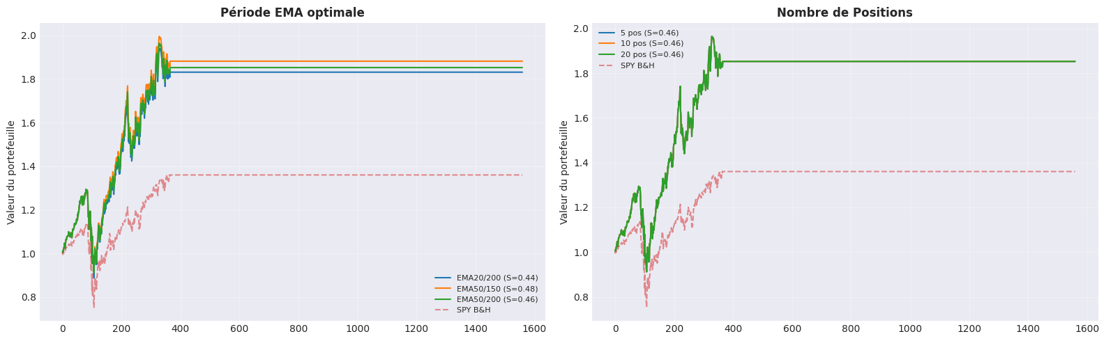
7. Visualisation des résultats

fig, axes = plt.subplots(1, 2, figsize=(16, 5))

# Gauche: EMA periods comparison
ax = axes[0]
for name, r in ema_results.items():
    ax.plot(r['cum'].values, label=f"{name} (S={r['sharpe']:.2f})", linewidth=1.5)
ax.plot(spy_values.values, label='SPY B&H', linestyle='--', alpha=0.5)
ax.set_title('Période EMA optimale', fontsize=12, fontweight='bold')
ax.set_ylabel('Valeur du portefeuille')
ax.legend(fontsize=8)
ax.grid(True, alpha=0.3)

# Droite: Position count comparison
ax = axes[1]
for name, r in pos_results.items():
    ax.plot(r['cum'].values, label=f"{name} pos (S={r['sharpe']:.2f})", linewidth=1.5)
ax.plot(spy_values.values, label='SPY B&H', linestyle='--', alpha=0.5)
ax.set_title('Nombre de Positions', fontsize=12, fontweight='bold')
ax.set_ylabel('Valeur du portefeuille')
ax.legend(fontsize=8)
ax.grid(True, alpha=0.3)

plt.tight_layout()
plt.savefig('trend_following_analysis.png', dpi=150, bbox_inches='tight')
plt.show()
print("Graphique sauvegardé.")

Graphique sauvegardé.

8. Conclusions et recommandations

Résumé

Métrique Meilleure config
Période EMA (à remplir)
Max Positions (à remplir)
Sharpe (à remplir)
CAGR (à remplir)

Verdict

Si Sharpe > 1.2: Déployer avec les paramètres optimaux

Points forts Trend Following

  • Diversification: 200 stocks réduit le risque spécifique
  • Adaptatif: Chaque stock a son propre cycle de tendance
  • Exécution: VWAP réduit le slippage

Limitations

  • Complexité: Nécessite un Alpha Model custom
  • Rebalancing fréquent: Quotidien = coûts de transaction
  • Whipsaws: Marchés range génèrent des faux signaux

Prochaines étapes

  1. Déployer sur QC cloud avec les paramètres optimaux
  2. Implémenter le custom Alpha Model complet
  3. Optimiser la universe sélection (liquidity filters)
  4. Tester avec Insight Weighting vs Equal Weight
Retour au sommet