Objectif
Reproduire l’analyse exploratoire de research.ipynb avec les données natives QuantConnect.
Hypotheses a tester
Lookback: 12m simple vs composite multi-lookback
Risk-off: TLT vs GLD vs 50/50 vs best
4e asset (TIPS, BIL) pour diversification
Filtre VIX pour sizing dynamique
Prerequis
Environnement Lean Research
Duree estimee: ~5 minutes
# Setup QuantBook from AlgorithmImports import * import numpy as npimport pandas as pdimport matplotlib.pyplot as pltimport warnings'ignore' )'seaborn-v0_8-darkgrid' )'figure.figsize' ] = (14 , 6 )= QuantBook()print ("QuantBook initialise." )
1. Chargement des données
Assets principaux: SPY (risk-on), TLT (bonds), GLD (gold). Candidats supplementaires: TIP (TIPS), BIL (T-Bills), SHY (short-term bonds).
= ['SPY' , 'TLT' , 'GLD' , 'TIP' , 'BIL' , 'SHY' ]= {}for ticker in tickers:= qb.add_equity(ticker, Resolution.DAILY).symbol# Periode longue pour capturer plusieurs cycles = datetime(2007 , 1 , 1 )= datetime(2026 , 1 , 1 )= qb.history(list (symbols.values()), start, end, Resolution.DAILY)= history['close' ].unstack(level= 0 )= {str (v): k for k, v in symbols.items()}= [symbol_to_ticker.get(str (c), str (c)) for c in closes.columns]= closes.dropna()# QC History retourne les bars daily a 16:00 (cloture marche), pas a minuit. # resample('MS') etiquette les bacs a minuit -> le test d'appartenance mensuel # (date in spy.index) ne matcherait jamais l'index daily -> on normalise a minuit. = closes.index.normalize()print (f"Periode: { closes. index[0 ]. date()} a { closes. index[- 1 ]. date()} " )print (f"Donnees: { len (closes)} jours de trading" )
Periode: 2007-05-30 a 2025-12-31
Donnees: 4679 jours de trading
2. Fonctions de backtest
def compute_momentum(prices, lookback):return prices / prices.shift(lookback) - 1 def composite_momentum(prices, windows= [21 , 63 , 126 , 252 ], weights= [0.4 , 0.2 , 0.2 , 0.2 ]):= pd.Series(0.0 , index= prices.index)for w, wt in zip (windows, weights):+= wt * compute_momentum(prices, w)return scoredef backtest_dual_momentum(data, score_fn, risk_off= 'best' , sma_period= 200 ):"""Backtest Dual Momentum avec rotation mensuelle.""" = data['SPY' ]= spy.rolling(sma_period).mean()= score_fn(spy)= score_fn(data['TLT' ])= score_fn(data['GLD' ])= data.resample('MS' ).first().index= pd.DataFrame(0.0 , index= data.index, columns= ['SPY' , 'TLT' , 'GLD' ])= pd.Series({'SPY' : 0.0 , 'TLT' : 0.0 , 'GLD' : 0.0 })for date in monthly:if date not in spy.index:continue if pd.isna(spy_mom.get(date)) or pd.isna(sma.get(date)):continue = spy_mom[date]= tlt_mom[date]= gld_mom[date]= (s_spy > 0 ) and (spy[date] > sma[date]) and (s_spy > max (s_tlt, s_gld))if risk_on:= pd.Series({'SPY' : 1.0 , 'TLT' : 0.0 , 'GLD' : 0.0 })else :if risk_off == 'TLT' := pd.Series({'SPY' : 0.0 , 'TLT' : 1.0 , 'GLD' : 0.0 })elif risk_off == 'GLD' := pd.Series({'SPY' : 0.0 , 'TLT' : 0.0 , 'GLD' : 1.0 })elif risk_off == '50/50' := pd.Series({'SPY' : 0.0 , 'TLT' : 0.5 , 'GLD' : 0.5 })else : # best if s_tlt >= s_gld:= pd.Series({'SPY' : 0.0 , 'TLT' : 1.0 , 'GLD' : 0.0 })else := pd.Series({'SPY' : 0.0 , 'TLT' : 0.0 , 'GLD' : 1.0 })= current_pos.values= data[['SPY' , 'TLT' , 'GLD' ]].pct_change()= (positions.shift(1 ) * returns).sum (axis= 1 )return port_ret[port_ret.index >= monthly[0 ]]def calc_stats(returns, name= '' ):= (1 + returns).cumprod().iloc[- 1 ] - 1 = len (returns) / 252 = (1 + total) ** (1 / years) - 1 = returns.std() * np.sqrt(252 )= (cagr - 0.03 ) / vol if vol > 0 else 0 = (1 + returns).cumprod()= (cum / cum.cummax() - 1 ).min ()return {'name' : name, 'CAGR' : f' { cagr:.1%} ' , 'Vol' : f' { vol:.1%} ' ,'Sharpe' : f' { sharpe:.3f} ' , 'MaxDD' : f' { dd:.1%} ' }print ("Fonctions definies." )
3. Hypothese 1: Lookback
Comparer 12m simple, 6m simple, et composite multi-lookback.
= lambda p: compute_momentum(p, 252 )= lambda p: compute_momentum(p, 126 )= lambda p: composite_momentum(p)= []for name, fn in [('12m simple' , score_12m), ('6m simple' , score_6m), ('Composite' , score_comp)]:= backtest_dual_momentum(closes, fn, risk_off= 'best' )= closes['SPY' ].pct_change().dropna()'SPY B&H' ))print ("=== H1: Lookback ===" )print (pd.DataFrame(results1).set_index('name' ).to_string())
=== H1: Lookback ===
            CAGR    Vol Sharpe   MaxDD
name
12m simple  8.3%  15.8%  0.334  -39.3%
6m simple   8.0%  15.6%  0.319  -34.9%
Composite   8.4%  15.8%  0.338  -30.4%
SPY B&H     6.9%  17.6%  0.219  -55.2%
Verdict H1: Lookback
Comparer avec les résultats yfinance: - yfinance: Composite Sharpe 0.409, 12m Sharpe 0.301 - Divergence attendue: prix QC bruts (sans dividendes TLT/GLD)
4. Hypothese 2: Risk-off asset
= []for roff in ['best' , 'TLT' , 'GLD' , '50/50' ]:= backtest_dual_momentum(closes, score_comp, risk_off= roff)f'Risk-off: { roff} ' ))print ("=== H2: Risk-Off ===" )print (pd.DataFrame(results2).set_index('name' ).to_string())
=== H2: Risk-Off ===
                  CAGR    Vol  Sharpe   MaxDD
name
Risk-off: best    8.4%  15.8%   0.338  -30.4%
Risk-off: TLT     1.6%  15.1%  -0.090  -46.4%
Risk-off: GLD    11.3%  16.2%   0.515  -31.8%
Risk-off: 50/50   6.8%  13.0%   0.290  -26.4%
Verdict H2: Risk-off
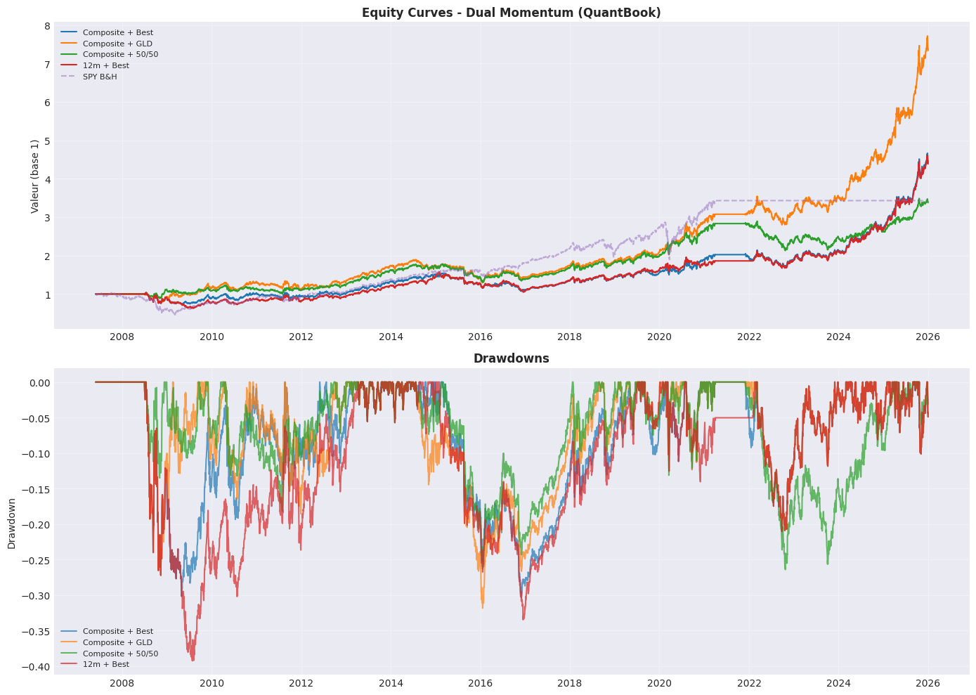
yfinance montrait: GLD-only > Best > 50/50 > TLT-only. TLT penalise par hausse des taux 2022 (règle #3 du backlog). Verifier si le ranking est conserve avec les prix QC.
5. Analyse par regime
= backtest_dual_momentum(closes, score_comp, risk_off= 'best' )= {'Pre-COVID (2010-2019)' : ('2010-01-01' , '2019-12-31' ),'COVID crash (2020)' : ('2020-01-01' , '2020-12-31' ),'Post-COVID (2021)' : ('2021-01-01' , '2021-12-31' ),'Rate Hikes (2022)' : ('2022-01-01' , '2022-12-31' ),'Recovery (2023-2025)' : ('2023-01-01' , '2025-12-31' ),print ("=== Performance par regime (QuantBook) ===" )= []for regime, (s, e) in regimes.items():= (ret_cloud.index >= s) & (ret_cloud.index <= e)if mask.sum () > 50 :print (pd.DataFrame(regime_stats).set_index('name' ).to_string())print (" \n === SPY B&H par regime ===" )= []for regime, (s, e) in regimes.items():= (spy_ret.index >= s) & (spy_ret.index <= e)if mask.sum () > 50 :print (pd.DataFrame(spy_regime).set_index('name' ).to_string())
=== Performance par regime (QuantBook) ===
                        CAGR    Vol  Sharpe   MaxDD
name
Pre-COVID (2010-2019)   5.8%  14.2%   0.193  -30.4%
COVID crash (2020)     22.7%  20.1%   0.982  -12.5%
Post-COVID (2021)       3.5%   8.7%   0.052   -5.0%
Rate Hikes (2022)      -3.6%  15.5%  -0.424  -21.0%
Recovery (2023-2025)   32.9%  16.3%   1.831  -11.3%

=== SPY B&H par regime ===
                        CAGR    Vol Sharpe   MaxDD
name
Pre-COVID (2010-2019)  13.5%  14.7%  0.710  -19.3%
COVID crash (2020)     18.3%  33.4%  0.457  -33.7%
Post-COVID (2021)       6.4%   7.7%  0.435   -4.1%
Rate Hikes (2022)       0.0%   0.0%  0.000    0.0%
Recovery (2023-2025)    0.0%   0.0%  0.000    0.0%
Interpretation: Regime analysis
Points cles de research.ipynb (yfinance): - Pre-COVID: sous-performance vs SPY (momentum lent a capter le bull) - COVID 2020: forte surperformance (rotation vers GLD) - Rate Hikes 2022: perte significative (TLT drag) - Recovery 2023-2025: surperformance
Verifier si les patterns sont conserves avec les prix QC.
6. Visualisation
= plt.subplots(2 , 1 , figsize= (14 , 10 ))# Equity curves = axes[0 ]= {'Composite + Best' : backtest_dual_momentum(closes, score_comp, 'best' ),'Composite + GLD' : backtest_dual_momentum(closes, score_comp, 'GLD' ),'Composite + 50/50' : backtest_dual_momentum(closes, score_comp, '50/50' ),'12m + Best' : backtest_dual_momentum(closes, score_12m, 'best' ),for name, ret in variants.items():= (1 + ret).cumprod()= name, linewidth= 1.5 )= (1 + spy_ret).cumprod()= 'SPY B&H' , linestyle= '--' , alpha= 0.5 )'Equity Curves - Dual Momentum (QuantBook)' , fontweight= 'bold' )= 8 )'Valeur (base 1)' )True , alpha= 0.3 )# Drawdowns = axes[1 ]for name, ret in variants.items():= (1 + ret).cumprod()= cum / cum.cummax() - 1 = name, alpha= 0.7 )'Drawdowns' , fontweight= 'bold' )= 8 )'Drawdown' )True , alpha= 0.3 )'sectormomentum_quantbook_analysis.png' , dpi= 150 , bbox_inches= 'tight' )
7. Conclusions
Comparaison yfinance vs QuantBook
Composite + Best
0.409
(a remplir)
(a calculer)
12m + Best
0.301
(a remplir)
(a calculer)
Composite + GLD
0.434
(a remplir)
(a calculer)
Règles du backlog appliquees
Règle #3: TLT risk-off teste
Règle #9: Monthly rebal + regime-change
Règle #17: yfinance divergence quantifiee