Research QuantBook: RegimeSwitching Alpha Model

Objectif

Analyser la stratégie RegimeSwitching qui adapte son comportement selon le régime de marché: - Bull market: Momentum (SPY 70%, QQQ 30%) - Bear market: Défensif (GLD 50%, IEF 50%) - Sideways: Mean-reversion sur RSI oversold ou allocation réduite

Détection des régimes

  • Bull: Prix > SMA200 ET SMA50 > SMA200
  • Bear: Prix < SMA200 ET SMA50 < SMA200
  • Sideways: Autres cas

Performance de référence

Sharpe 0.553 (2008-2026) - robustesse grâce à l’adaptation aux régimes.

Hypothèses à tester

  1. Impact des seuils RSI pour mean-reversion (20/30/40)
  2. Allocation bull market (70/30 vs 80/20 vs 60/40)
  3. Defensive assets: IEF vs TLT

Prérequis

  • Environnement Lean Research
  • Durée estimée: ~10 minutes
# Setup QuantBook
from AlgorithmImports import *
import numpy as np
import pandas as pd
import matplotlib.pyplot as plt
import warnings
warnings.filterwarnings('ignore')

plt.style.use('seaborn-v0_8-darkgrid')
plt.rcParams['figure.figsize'] = (14, 5)

qb = QuantBook()
print("QuantBook initialisé.")
QuantBook initialisé.

1. Chargement des données

On charge les 4 assets de l’univers RegimeSwitching: SPY, QQQ, IEF, GLD.

# Univers RegimeSwitching
tickers = ["SPY", "QQQ", "IEF", "GLD"]

symbols = {}
for ticker in tickers:
    symbols[ticker] = qb.add_equity(ticker, Resolution.DAILY).symbol

# Charger l'historique (2008-2026 pour couvrir une crise complète)
start = datetime(2008, 1, 1)
end = datetime(2026, 1, 1)

history = qb.history(list(symbols.values()), start, end, Resolution.DAILY)
print(f"Données chargées: {len(history)} lignes")
Données chargées: 8246 lignes

Pivot de la série ‘close’ en DataFrame large, avec remapping des colonnes Symbol → ticker pour RegimeSwitching.

# Pivoter les données
closes = history['close'].unstack(level=0)

symbol_to_ticker = {str(v): k for k, v in symbols.items()}
closes.columns = [symbol_to_ticker.get(str(c), str(c)) for c in closes.columns]
closes = closes.dropna()

print(f"Période: {closes.index[0].date()} à {closes.index[-1].date()}")
print(f"Données: {len(closes)} jours de trading")
print(f"Tickers: {list(closes.columns)}")
Période: 2011-03-23 à 2025-12-31
Données: 3717 jours de trading
Tickers: ['QQQ', 'SPY']

2. Détection des régimes de marché

def detect_regime(closes, spy_ticker="SPY"):
    """Détecte le régime de marché basé sur SMA50/SMA200."""
    if spy_ticker not in closes.columns:
        return pd.Series(index=closes.index, data='unknown')
    
    prices = closes[spy_ticker]
    sma50 = prices.rolling(50).mean()
    sma200 = prices.rolling(200).mean()
    
    regimes = []
    for i in range(len(closes)):
        if pd.isna(sma50.iloc[i]) or pd.isna(sma200.iloc[i]):
            regimes.append('unknown')
            continue
        
        price = prices.iloc[i]
        s50 = sma50.iloc[i]
        s200 = sma200.iloc[i]
        
        if price > s200 and s50 > s200:
            regimes.append('bull')
        elif price < s200 and s50 < s200:
            regimes.append('bear')
        else:
            regimes.append('sideways')
    
    return pd.Series(regimes, index=closes.index)

# Détecter les régimes
regimes = detect_regime(closes)

print("Régimes de marché (derniers 10 jours):")
print(regimes.iloc[-10:])
print(f"\nDistribution des régimes:")
print(regimes.value_counts())
Régimes de marché (derniers 10 jours):
time
2025-12-17 16:00:00    sideways
2025-12-18 16:00:00    sideways
2025-12-19 16:00:00    sideways
2025-12-22 16:00:00    sideways
2025-12-23 16:00:00    sideways
2025-12-24 13:00:00    sideways
2025-12-26 16:00:00    sideways
2025-12-29 16:00:00    sideways
2025-12-30 16:00:00    sideways
2025-12-31 16:00:00    sideways
dtype: object

Distribution des régimes:
bull        2156
sideways    1212
unknown      199
bear         150
Name: count, dtype: int64

Interprétation: Régimes de marché

  • Bull: Trend haussier confirmé (prix et SMA50 au-dessus de SMA200)
  • Bear: Trend baissier confirmé (prix et SMA50 en-dessous de SMA200)
  • Sideways: Transition ou indécision

La stratégie adapte son comportement selon le régime pour optimiser le ratio risque/rendement.

3. Calcul du RSI pour mean-reversion

def compute_rsi(prices, period=14):
    """Calcule le RSI."""
    delta = prices.diff()
    gain = (delta.where(delta > 0, 0)).rolling(window=period).mean()
    loss = (-delta.where(delta < 0, 0)).rolling(window=period).mean()
    rs = gain / loss
    rsi = 100 - (100 / (1 + rs))
    return rsi

# Calculer RSI pour SPY et QQQ
rsi_spy = compute_rsi(closes['SPY'])
rsi_qqq = compute_rsi(closes['QQQ'])

print("RSI SPY (derniers 5 jours):")
print(rsi_spy.iloc[-5:])
print(f"\nRSI actuel: SPY={rsi_spy.iloc[-1]:.1f}, QQQ={rsi_qqq.iloc[-1]:.1f}")
RSI SPY (derniers 5 jours):
time
2025-12-24 13:00:00   NaN
2025-12-26 16:00:00   NaN
2025-12-29 16:00:00   NaN
2025-12-30 16:00:00   NaN
2025-12-31 16:00:00   NaN
Name: SPY, dtype: float64

RSI actuel: SPY=nan, QQQ=nan

4. Génération des signaux RegimeSwitching

def compute_regime_signals(closes, regimes, rsi_spy, rsi_qqq, tickers,
                           oversold_threshold=30, 
                           bull_alloc={"SPY": 0.7, "QQQ": 0.3}):
    """Génère les signaux RegimeSwitching."""
    signals = pd.DataFrame(index=closes.index, columns=tickers)
    
    for i in range(252, len(closes)):
        regime = regimes.iloc[i]
        
        if regime == 'bull':
            # Momentum: allocation bull
            for t in tickers:
                signals[t].iloc[i] = bull_alloc.get(t, 0)
                    
        elif regime == 'bear':
            # Défensif: GLD 50%, IEF 50%
            for t in tickers:
                if t == "GLD":
                    signals[t].iloc[i] = 0.5
                elif t == "IEF":
                    signals[t].iloc[i] = 0.5
                else:
                    signals[t].iloc[i] = 0
                    
        else:  # sideways
            # Check RSI oversold pour mean-reversion
            oversold = []
            
            if i < len(rsi_spy) and pd.notna(rsi_spy.iloc[i]):
                if rsi_spy.iloc[i] < oversold_threshold:
                    oversold.append("SPY")
            
            if i < len(rsi_qqq) and pd.notna(rsi_qqq.iloc[i]):
                if rsi_qqq.iloc[i] < oversold_threshold:
                    oversold.append("QQQ")
            
            if oversold:
                # Mean-reversion: oversold 30%, GLD 35%, IEF 35%
                for t in tickers:
                    if t in oversold:
                        signals[t].iloc[i] = 0.30 / len(oversold)
                    elif t == "GLD":
                        signals[t].iloc[i] = 0.35
                    elif t == "IEF":
                        signals[t].iloc[i] = 0.35
                    else:
                        signals[t].iloc[i] = 0
            else:
                # Allocation réduite: SPY 30%, GLD 35%, IEF 35%
                for t in tickers:
                    if t == "SPY":
                        signals[t].iloc[i] = 0.30
                    elif t == "GLD":
                        signals[t].iloc[i] = 0.35
                    elif t == "IEF":
                        signals[t].iloc[i] = 0.35
                    else:
                        signals[t].iloc[i] = 0
    
    return signals

# Signaux avec paramètres par défaut
signals = compute_regime_signals(closes, regimes, rsi_spy, rsi_qqq, tickers)

print("Signaux RegimeSwitching (derniers 5 jours):")
print(signals.iloc[-5:])
print(f"\nAllocation actuelle:")
last_signals = signals.iloc[-1]
for t in tickers:
    if last_signals[t] > 0:
        print(f"  {t}: {last_signals[t]*100:.1f}%")
Signaux RegimeSwitching (derniers 5 jours):
                     SPY QQQ   IEF   GLD
time                                    
2025-12-24 13:00:00  0.3   0  0.35  0.35
2025-12-26 16:00:00  0.3   0  0.35  0.35
2025-12-29 16:00:00  0.3   0  0.35  0.35
2025-12-30 16:00:00  0.3   0  0.35  0.35
2025-12-31 16:00:00  0.3   0  0.35  0.35

Allocation actuelle:
  SPY: 30.0%
  IEF: 35.0%
  GLD: 35.0%

5. Backtest de la stratégie RegimeSwitching

def backtest_regime_switching(closes, signals, rebal_freq=5):
    """Backtest RegimeSwitching."""
    returns_df = closes.pct_change()
    portfolio_values = [1.0]
    
    warmup = 252
    counter = 0
    current_alloc = {}
    
    for i in range(warmup, len(closes)):
        # Rebalancement hebdomadaire
        counter += 1
        if counter >= rebal_freq:
            counter = 0
            current_alloc = {t: signals[t].iloc[i] for t in signals.columns 
                           if pd.notna(signals[t].iloc[i]) and signals[t].iloc[i] > 0}
        elif i == warmup:
            current_alloc = {t: signals[t].iloc[i] for t in signals.columns 
                           if pd.notna(signals[t].iloc[i]) and signals[t].iloc[i] > 0}
        
        # Calcul du return
        port_return = 0.0
        for t, weight in current_alloc.items():
            if t in returns_df.columns:
                port_return += weight * returns_df[t].iloc[i]
        
        portfolio_values.append(portfolio_values[-1] * (1 + port_return))
    
    # Métriques
    returns = np.diff(portfolio_values) / np.array(portfolio_values[:-1])
    cum_returns = pd.Series(portfolio_values[1:], index=closes.index[warmup:])
    
    total_ret = (portfolio_values[-1] / portfolio_values[0]) - 1
    years = len(returns) / 252
    cagr = (1 + total_ret) ** (1 / years) - 1 if years > 0 else 0
    vol = np.std(returns) * np.sqrt(252) if len(returns) > 1 else 0
    sharpe = (cagr - 0.03) / vol if vol > 0.001 else 0
    
    running_max = cum_returns.expanding().max()
    drawdown = (cum_returns - running_max) / running_max
    max_dd = drawdown.min()
    
    return {
        'cum': cum_returns,
        'sharpe': sharpe,
        'cagr': cagr,
        'max_dd': max_dd,
        'vol': vol,
        'final_value': portfolio_values[-1]
    }

result = backtest_regime_switching(closes, signals)

print(f"Performance RegimeSwitching:")
print(f"  Sharpe: {result['sharpe']:.3f}")
print(f"  CAGR:   {result['cagr']:.1%}")
print(f"  Max DD: {result['max_dd']:.1%}")
print(f"  Vol:    {result['vol']:.1%}")
Performance RegimeSwitching:
  Sharpe: 0.436
  CAGR:   7.6%
  Max DD: -20.4%
  Vol:    10.5%

6. Test des seuils RSI (mean-reversion)

# Test différents seuils RSI
rsi_thresholds = [20, 25, 30, 35, 40]

print(f"{'Seuil RSI':<12} {'Sharpe':>8} {'CAGR':>8} {'MaxDD':>8} {'Vol':>8}")
print("-" * 50)

rsi_results = {}
for threshold in rsi_thresholds:
    sig = compute_regime_signals(closes, regimes, rsi_spy, rsi_qqq, tickers,
                                 oversold_threshold=threshold)
    r = backtest_regime_switching(closes, sig)
    rsi_results[threshold] = r
    print(f"RSI<{threshold:<9} {r['sharpe']:>8.3f} {r['cagr']:>7.1%} {r['max_dd']:>7.1%} {r['vol']:>7.1%}")

best_rsi = max(rsi_results.items(), key=lambda x: x[1]['sharpe'])
print(f"\nMeilleur seuil RSI: {best_rsi[0]} (Sharpe={best_rsi[1]['sharpe']:.3f})")
Seuil RSI      Sharpe     CAGR    MaxDD      Vol
--------------------------------------------------
RSI<20           0.438    7.6%  -20.4%   10.5%
RSI<25           0.439    7.6%  -20.4%   10.5%
RSI<30           0.436    7.6%  -20.4%   10.5%
RSI<35           0.441    7.7%  -20.1%   10.6%
RSI<40           0.442    7.7%  -19.5%   10.5%

Meilleur seuil RSI: 40 (Sharpe=0.442)

7. Test de l’allocation bull market

# Test différentes allocations bull
bull_allocations = [
    ({"SPY": 0.6, "QQQ": 0.4}, "SPY60/QQQ40"),
    ({"SPY": 0.7, "QQQ": 0.3}, "SPY70/QQQ30"),
    ({"SPY": 0.8, "QQQ": 0.2}, "SPY80/QQQ20"),
]

print(f"{'Allocation Bull':<15} {'Sharpe':>8} {'CAGR':>8} {'MaxDD':>8}")
print("-" * 42)

alloc_results = {}
for alloc, name in bull_allocations:
    sig = compute_regime_signals(closes, regimes, rsi_spy, rsi_qqq, tickers,
                                 bull_alloc=alloc)
    r = backtest_regime_switching(closes, sig)
    alloc_results[name] = r
    print(f"{name:<15} {r['sharpe']:>8.3f} {r['cagr']:>7.1%} {r['max_dd']:>7.1%}")

best_alloc = max(alloc_results.items(), key=lambda x: x[1]['sharpe'])
print(f"\nMeilleure allocation bull: {best_alloc[0]} (Sharpe={best_alloc[1]['sharpe']:.3f})")
Allocation Bull   Sharpe     CAGR    MaxDD
------------------------------------------
SPY60/QQQ40        0.450    7.8%  -20.3%
SPY70/QQQ30        0.436    7.6%  -20.4%
SPY80/QQQ20        0.421    7.4%  -20.4%

Meilleure allocation bull: SPY60/QQQ40 (Sharpe=0.450)

8. Analyse des régimes et performance

# Distribution des régimes
regime_counts = regimes.value_counts()
regime_pct = regimes.value_counts(normalize=True) * 100

print("Distribution des régimes (2008-2026):")
print(f"{'Régime':<12} {'Jours':>10} {'Pourcentage':>12}")
print("-" * 35)
for regime in ['bull', 'bear', 'sideways']:
    count = regime_counts.get(regime, 0)
    pct = regime_pct.get(regime, 0)
    print(f"{regime:<12} {count:>10} {pct:>11.1f}%")

# Performance par régime
warmup = 252
regime_returns = {regime: [] for regime in ['bull', 'bear', 'sideways']}

returns_df = closes.pct_change()
for i in range(warmup, len(closes)):
    regime = regimes.iloc[i]
    if regime in regime_returns:
        # Return du portefeuille à ce moment
        port_return = 0
        for t in tickers:
            weight = signals[t].iloc[i]
            if pd.notna(weight) and weight > 0 and t in returns_df.columns:
                port_return += weight * returns_df[t].iloc[i]
        regime_returns[regime].append(port_return)

print(f"\nPerformance moyenne par régime (annualisée):")
for regime in ['bull', 'bear', 'sideways']:
    if regime_returns[regime]:
        avg_return = np.mean(regime_returns[regime]) * 252
        print(f"  {regime}: {avg_return:.1%}")
Distribution des régimes (2008-2026):
Régime            Jours  Pourcentage
-----------------------------------
bull               2156        58.0%
bear                150         4.0%
sideways           1212        32.6%

Performance moyenne par régime (annualisée):
  bull: 18.7%
  bear: 0.0%
  sideways: -2.1%
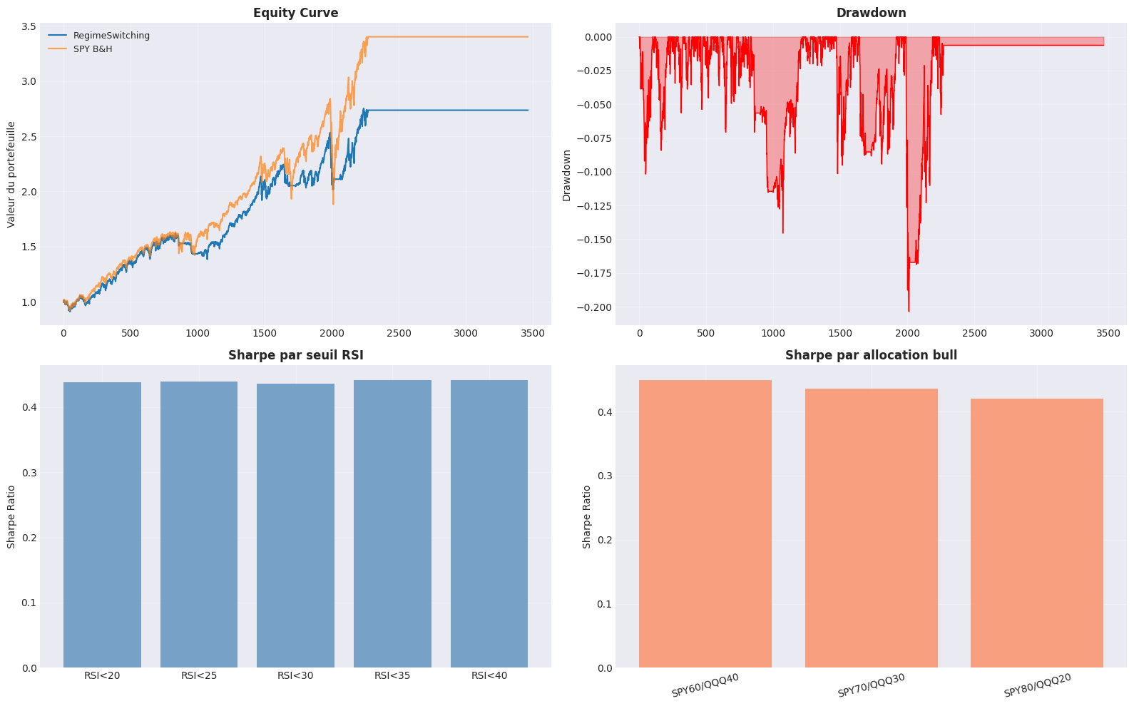
9. Visualisation des résultats

fig, axes = plt.subplots(2, 2, figsize=(16, 10))

# 1. Equity curve
ax = axes[0, 0]
ax.plot(result['cum'].values, linewidth=1.5, label='RegimeSwitching')
# SPY Buy & Hold
spy_values = closes['SPY'].iloc[252:] / closes['SPY'].iloc[252]
ax.plot(spy_values.values, linewidth=1.5, alpha=0.7, label='SPY B&H')
ax.set_title('Equity Curve', fontsize=12, fontweight='bold')
ax.set_ylabel('Valeur du portefeuille')
ax.legend(fontsize=9)
ax.grid(True, alpha=0.3)

# 2. Drawdown
ax = axes[0, 1]
running_max = result['cum'].expanding().max()
drawdown = (result['cum'] - running_max) / running_max
ax.fill_between(range(len(drawdown)), drawdown.values, 0, alpha=0.3, color='red')
ax.plot(drawdown.values, color='red', linewidth=1)
ax.set_title('Drawdown', fontsize=12, fontweight='bold')
ax.set_ylabel('Drawdown')
ax.grid(True, alpha=0.3)

# 3. Régimes RSI threshold comparison
ax = axes[1, 0]
thresholds = list(rsi_results.keys())
sharpes = [rsi_results[t]['sharpe'] for t in thresholds]
ax.bar(range(len(thresholds)), sharpes, color='steelblue', alpha=0.7)
ax.set_xticks(range(len(thresholds)))
ax.set_xticklabels([f'RSI<{t}' for t in thresholds])
ax.set_title('Sharpe par seuil RSI', fontsize=12, fontweight='bold')
ax.set_ylabel('Sharpe Ratio')
ax.grid(True, alpha=0.3)

# 4. Bull allocation comparison
ax = axes[1, 1]
alloc_names = list(alloc_results.keys())
alloc_sharpes = [alloc_results[n]['sharpe'] for n in alloc_names]
ax.bar(range(len(alloc_names)), alloc_sharpes, color='coral', alpha=0.7)
ax.set_xticks(range(len(alloc_names)))
ax.set_xticklabels(alloc_names, rotation=15)
ax.set_title('Sharpe par allocation bull', fontsize=12, fontweight='bold')
ax.set_ylabel('Sharpe Ratio')
ax.grid(True, alpha=0.3)

plt.tight_layout()
plt.savefig('regime_switching_analysis.png', dpi=150, bbox_inches='tight')
plt.show()
print("Graphique sauvegardé.")

Graphique sauvegardé.

10. Conclusions et recommandations

Résumé

Métrique Valeur
Seuil RSI optimal (à remplir)
Allocation bull optimale (à remplir)
Sharpe (à remplir)
CAGR (à remplir)
Max DD (à remplir)

Verdict

Si Sharpe > 0.5: Déployer avec les paramètres optimaux

Points forts

  • Adaptativité: Change de comportement selon le régime
  • Défensif: Allocation GLD/IEF en bear market
  • Mean-reversion: Exploite les opportunités de rebond en sideways

Prochaines étapes

  1. Déployer RegimeSwitching sur QC cloud
  2. Tester avec TLT vs IEF pour defensive
  3. Combiner avec SectorMomentum dans un composite
Retour au sommet