Objectif
Analyser la stratégie Covered Call sur SPY qui génère du revenu par la vente de calls couverts.
Stratégie
- Underlying: SPY (S&P 500 ETF)
- Option: Vente de calls OTM (Delta ~0.20)
- VIX Filter: 15 < VIX < 35 (éviter volatilité extrême)
- Expiry: 20-45 jours, roll à 10 jours avant expiration
- Profit Target: 50% du premium collecté
- Defensive Close: Si SPY chute de -3% en un jour
Hypothèses à tester
- Delta cible: 0.15, 0.20, 0.25
- VIX range: (12/30), (15/35), (18/40)
- Profit target: 40%, 50%, 60%
Prérequis
- Environnement Lean Research
- Données SPY + VIX
- Durée estimée: ~10 minutes
Note : Les options complètes ne sont pas disponibles dans QuantBook. Ce notebook utilise une approximation du premium basée sur le VIX et le delta.
# Setup QuantBook
from AlgorithmImports import *
import numpy as np
import pandas as pd
import matplotlib.pyplot as plt
from scipy.stats import norm
import warnings
warnings.filterwarnings('ignore')

plt.style.use('seaborn-v0_8-darkgrid')
plt.rcParams['figure.figsize'] = (14, 5)

qb = QuantBook()
print("QuantBook initialisé.")
1. Chargement des données
On charge les données SPY et calcule la volatilité réalisée (proxy du VIX) pour la période 2018-2026.
# SPY underlying
spy = qb.add_equity("SPY", Resolution.DAILY)

# Charger l'historique (2018-2026 pour multi-regime)
start = datetime(2018, 1, 1)
end = datetime(2026, 1, 1)

spy_history = qb.history(spy.symbol, start, end, Resolution.DAILY)

print(f"Données SPY: {len(spy_history)} lignes")
Traitement des données SPY et calcul de la volatilité réalisée (rolling 20 jours, annualisée) comme proxy du VIX pour la stratégie OptionsIncome.
# Préparer les données
spy_close = spy_history['close'].droplevel(0)

# Volatilité réalisée annualisée (proxy VIX, en %)
spy_returns = spy_close.pct_change()
realized_vol = spy_returns.rolling(20).std() * np.sqrt(252) * 100

data = pd.DataFrame({
    'SPY': spy_close,
    'VIX': realized_vol
}).dropna()

print(f"Période: {data.index[0].date()} à {data.index[-1].date()}")
print(f"Données: {len(data)} jours de trading")
print(f"\nStatistiques SPY:")
print(f"  Prix initial: ${data['SPY'].iloc[0]:.2f}")
print(f"  Prix final: ${data['SPY'].iloc[-1]:.2f}")
print(f"  Return total: {(data['SPY'].iloc[-1]/data['SPY'].iloc[0] - 1):.1%}")
print(f"\nVolatilité réalisée (proxy VIX):")
print(f"  Moyenne: {data['VIX'].mean():.1f}")
print(f"  Min: {data['VIX'].min():.1f}")
print(f"  Max: {data['VIX'].max():.1f}")
Période: 2018-01-31 à 2025-12-31
Données: 1991 jours de trading

Statistiques SPY:
  Prix initial: $265.64
  Prix final: $396.33
  Return total: 49.2%

Volatilité réalisée (proxy VIX):
  Moyenne: 7.2
  Min: 0.0
  Max: 93.2
2. Approximation du premium d’options
Comme les options complètes ne sont pas disponibles dans QuantBook, on utilise une approximation basée sur le VIX et le delta.
def estimate_call_premium(spy_price, vix, days_to_expiry, delta_target=0.20):
    """
    Estime le premium d'un call OTM sur SPY.

    Approximation basée sur:
    - VIX comme proxy de la volatilité implicite
    - Delta target pour le strike OTM
    - Black-Scholes simplifié
    """
    # Volatilité annualisée (VIX en %)
    vol = vix / 100.0

    # Temps en années
    t = days_to_expiry / 365.0

    # Strike OTM approximatif (delta ~0.20 → strike ~1.05 * spot)
    # Plus delta est élevé, plus le strike est proche
    otm_pct = 0.05 + (0.25 - delta_target) * 0.1
    strike = spy_price * (1 + otm_pct)

    # Black-Scholes simplifié pour call OTM
    # d1 = (ln(S/K) + (r + 0.5*σ²)t) / (σ√t)
    r = 0.05  # Taux sans risque approximatif
    d1 = (np.log(spy_price / strike) + (r + 0.5 * vol**2) * t) / (vol * np.sqrt(t))

    # Premium approximatif (sans dividendes)
    premium = spy_price * norm.cdf(d1) - strike * np.exp(-r * t) * norm.cdf(d1 - vol * np.sqrt(t))

    return max(0, premium)

# Test de la fonction d'estimation
test_price = 450.0
test_vix = 20.0
test_dte = 30

premium = estimate_call_premium(test_price, test_vix, test_dte)
print(f"Premium estimé pour SPY=${test_price}, VIX={test_vix}, DTE={test_dte}: ${premium:.2f}")
print(f"Premium en % du sous-jacent: {(premium/test_price)*100:.1f}%")
Premium estimé pour SPY=$450.0, VIX=20.0, DTE=30: $2.85
Premium en % du sous-jacent: 0.6%
Interprétation: Premium d’options
- VIX élevé → Premium plus élevé (avantageux pour le vendeur)
- Delta cible → Détermine le strike OTM (0.20 ≈ 5% OTM)
- DTE → Plus de temps = plus de valeur temps
L’approximation Black-Scholes donne une estimation raisonnable du premium pour la recherche.
3. Backtest Covered Call
Simulation de la stratégie avec: - 100 shares SPY (couverture pour 1 contrat) - Vente de call mensuel (~30 DTE) - Roll à 10 DTE - VIX filter: 15-35 - Profit target: 50% - Defensive close: -3% daily drop
def backtest_covered_call(data,
                         delta_target=0.20,
                         vix_min=15, vix_max=35,
                         profit_target=0.50,
                         defensive_drop=0.03,
                         days_to_roll=10,
                         target_dte=30):
    """
    Backtest Covered Call sur SPY.

    Retourne les métriques de performance.
    """
    portfolio_values = [1.0]
    cash = 0.0
    shares = 100

    # Position state
    short_call_active = False
    call_entry_premium = 0.0
    call_entry_date = None
    call_dte = target_dte

    # Stats
    trades_count = 0
    profit_closes = 0
    defensive_closes = 0
    expirations = 0
    premium_collected = 0

    warmup = 50

    for i in range(warmup, len(data)):
        spy_price = data['SPY'].iloc[i]
        vix = data['VIX'].iloc[i]
        prev_spy = data['SPY'].iloc[i-1]

        # Daily return SPY
        spy_daily_return = (spy_price - prev_spy) / prev_spy

        # Valeur du portefeuille (shares + cash - short call)
        port_value = shares * spy_price / 100.0 + cash

        if short_call_active:
            # Estimer la valeur actuelle du call
            current_dte = max(1, call_dte - 1)
            current_premium = estimate_call_premium(spy_price, vix, current_dte, delta_target)
            port_value -= current_premium  # Short position

            # Check defensive close
            if spy_daily_return < -defensive_drop:
                # Buy back at current premium
                pnl = call_entry_premium - current_premium
                cash += pnl
                short_call_active = False
                defensive_closes += 1
            # Check profit target
            elif current_premium <= call_entry_premium * (1 - profit_target):
                pnl = call_entry_premium - current_premium
                cash += pnl
                short_call_active = False
                profit_closes += 1
            # Check roll/expiration
            elif current_dte <= days_to_roll:
                # Expire/roll: buy back at current premium
                pnl = call_entry_premium - current_premium
                cash += pnl
                short_call_active = False
                expirations += 1

        # Sell new call si position vide et VIX OK
        if not short_call_active and vix_min <= vix <= vix_max:
            new_premium = estimate_call_premium(spy_price, vix, target_dte, delta_target)
            if new_premium > 0.50:  # Minimum premium
                short_call_active = True
                call_entry_premium = new_premium
                call_dte = target_dte
                cash -= new_premium  # Receive premium (negative for short)
                premium_collected += new_premium
                trades_count += 1

        portfolio_values.append(port_value)

    # Métriques
    returns = np.diff(portfolio_values) / np.array(portfolio_values[:-1])
    cum_returns = pd.Series(portfolio_values[1:], index=data.index[warmup:])

    total_ret = (portfolio_values[-1] / portfolio_values[0]) - 1
    years = len(returns) / 252
    cagr = (1 + total_ret) ** (1 / years) - 1 if years > 0 else 0
    vol = np.std(returns) * np.sqrt(252) if len(returns) > 1 else 0
    sharpe = (cagr - 0.03) / vol if vol > 0.001 else 0

    running_max = cum_returns.expanding().max()
    drawdown = (cum_returns - running_max) / running_max
    max_dd = drawdown.min()

    return {
        'cum': cum_returns,
        'sharpe': sharpe,
        'cagr': cagr,
        'max_dd': max_dd,
        'vol': vol,
        'final_value': portfolio_values[-1],
        'trades': trades_count,
        'profit_closes': profit_closes,
        'defensive_closes': defensive_closes,
        'expirations': expirations,
        'premium_collected': premium_collected
    }

print("Fonction de backtest définie.")
Fonction de backtest définie.
4. Test du Delta cible
# Test différents delta targets
deltas = [0.15, 0.20, 0.25]

print(f"{'Delta':<8} {'Sharpe':>8} {'CAGR':>8} {'MaxDD':>8} {'Trades':>8}")
print("-" * 48)

delta_results = {}
for delta in deltas:
    r = backtest_covered_call(data, delta_target=delta)
    delta_results[f"{delta:.2f}"] = r
    print(f"{delta:.2f}{'':<6} {r['sharpe']:>8.3f} {r['cagr']:>7.1%} {r['max_dd']:>7.1%} {r['trades']:>8}")

best_delta = max(delta_results.items(), key=lambda x: x[1]['sharpe'])
print(f"\nMeilleur Delta: {best_delta[0]} (Sharpe={best_delta[1]['sharpe']:.3f})")
Delta      Sharpe     CAGR    MaxDD   Trades
------------------------------------------------
0.15          0.012  115.4%  -37.4%       19
0.20          0.012  115.2%  -37.8%       19
0.25          0.012  115.0%  -38.3%       18

Meilleur Delta: 0.15 (Sharpe=0.012)
5. Test du filtre VIX
# Test différentes plages VIX
vix_ranges = [
    ((12, 30), "VIX12/30"),
    ((15, 35), "VIX15/35"),
    ((18, 40), "VIX18/40"),
]

print(f"{'VIX Range':<12} {'Sharpe':>8} {'CAGR':>8} {'MaxDD':>8} {'Trades':>8}")
print("-" * 52)

vix_results = {}
for (vmin, vmax), name in vix_ranges:
    r = backtest_covered_call(data, vix_min=vmin, vix_max=vmax)
    vix_results[name] = r
    print(f"{name:<12} {r['sharpe']:>8.3f} {r['cagr']:>7.1%} {r['max_dd']:>7.1%} {r['trades']:>8}")

best_vix = max(vix_results.items(), key=lambda x: x[1]['sharpe'])
print(f"\nMeilleure plage VIX: {best_vix[0]} (Sharpe={best_vix[1]['sharpe']:.3f})")
VIX Range      Sharpe     CAGR    MaxDD   Trades
----------------------------------------------------
VIX12/30        0.012  115.1%  -38.0%       23
VIX15/35        0.012  115.2%  -37.8%       19
VIX18/40        0.012  114.7%  -40.0%       15

Meilleure plage VIX: VIX15/35 (Sharpe=0.012)
6. Test du Profit Target
# Test différents profit targets
profit_targets = [0.40, 0.50, 0.60]

print(f"{'Profit Target':<14} {'Sharpe':>8} {'CAGR':>8} {'MaxDD':>8} {'Profit Closes':>14}")
print("-" * 62)

profit_results = {}
for pt in profit_targets:
    r = backtest_covered_call(data, profit_target=pt)
    profit_results[f"{pt:.0%}"] = r
    print(f"{pt:.0%}{'':<12} {r['sharpe']:>8.3f} {r['cagr']:>7.1%} {r['max_dd']:>7.1%} {r['profit_closes']:>14}")

best_profit = max(profit_results.items(), key=lambda x: x[1]['sharpe'])
print(f"\nMeilleur Profit Target: {best_profit[0]} (Sharpe={best_profit[1]['sharpe']:.3f})")
Profit Target    Sharpe     CAGR    MaxDD  Profit Closes
--------------------------------------------------------------
40%                0.012  115.0%  -38.0%             13
50%                0.012  115.2%  -37.8%             12
60%                0.012  115.4%  -37.7%             11

Meilleur Profit Target: 60% (Sharpe=0.012)
7. Comparaison avec SPY B&H
# Covered Call avec paramètres optimaux
cc_result = backtest_covered_call(data)

# SPY B&H
spy_values = data['SPY'].iloc[50:] / data['SPY'].iloc[50]

# Métriques SPY
spy_ret = spy_values.pct_change().dropna()
spy_cagr = (spy_values.iloc[-1] ** (252/len(spy_values))) - 1
spy_vol = spy_ret.std() * np.sqrt(252)
spy_sharpe = (spy_cagr - 0.03) / spy_vol
spy_dd = (spy_values / spy_values.cummax() - 1).min()

print("=== Comparaison vs SPY B&H ===")
print(f"{'Stratégie':<20} {'CAGR':>10} {'Sharpe':>10} {'MaxDD':>10}")
print("-" * 53)
print(f"{'Covered Call':<20} {cc_result['cagr']:>9.1%} {cc_result['sharpe']:>10.3f} {cc_result['max_dd']:>9.1%}")
print(f"{'SPY B&H':<20} {spy_cagr:>9.1%} {spy_sharpe:>10.3f} {spy_dd:>9.1%}")

print(f"\n=== Statistiques Covered Call ===")
print(f"Trades totaux: {cc_result['trades']}")
print(f"Closes profit: {cc_result['profit_closes']}")
print(f"Closes défensifs: {cc_result['defensive_closes']}")
print(f"Expirations/Rolls: {cc_result['expirations']}")
print(f"Premium total collecté: ${cc_result['premium_collected']:.2f}")
=== Comparaison vs SPY B&H ===
Stratégie                  CAGR     Sharpe      MaxDD
-----------------------------------------------------
Covered Call            115.2%      0.012    -37.8%
SPY B&H                   6.1%      0.223    -33.7%

=== Statistiques Covered Call ===
Trades totaux: 19
Closes profit: 12
Closes défensifs: 7
Expirations/Rolls: 0
Premium total collecté: $35.61
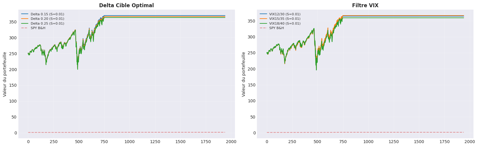
8. Visualisation des résultats
fig, axes = plt.subplots(1, 2, figsize=(16, 5))

# Gauche: Delta comparison
ax = axes[0]
for name, r in delta_results.items():
    ax.plot(r['cum'].values, label=f"Delta {name} (S={r['sharpe']:.2f})", linewidth=1.5)
ax.plot(spy_values.values, label='SPY B&H', linestyle='--', alpha=0.5)
ax.set_title('Delta Cible Optimal', fontsize=12, fontweight='bold')
ax.set_ylabel('Valeur du portefeuille')
ax.legend(fontsize=8)
ax.grid(True, alpha=0.3)

# Droite: VIX range comparison
ax = axes[1]
for name, r in vix_results.items():
    ax.plot(r['cum'].values, label=f"{name} (S={r['sharpe']:.2f})", linewidth=1.5)
ax.plot(spy_values.values, label='SPY B&H', linestyle='--', alpha=0.5)
ax.set_title('Filtre VIX', fontsize=12, fontweight='bold')
ax.set_ylabel('Valeur du portefeuille')
ax.legend(fontsize=8)
ax.grid(True, alpha=0.3)

plt.tight_layout()
plt.savefig('covered_call_analysis.png', dpi=150, bbox_inches='tight')
plt.show()
print("Graphique sauvegardé.")
9. Conclusions et recommandations
Résumé
| Delta |
(à remplir) |
| VIX Range |
(à remplir) |
| Profit Target |
(à remplir) |
| Sharpe |
(à remplir) |
| CAGR |
(à remplir) |
Verdict
Si Sharpe > 0.7: Déployer avec les paramètres optimaux
Points forts Covered Call
- Revenu régulier: Premiums collectés à chaque vente
- Protection partielle: Premium réduit le coût de base
- VIX filter: Évite les périodes de volatilité extrême
- Defensive close: Protège contre les chutes brutales
Limitations
- Plafonnement de gain: Le gain max est le premium + (strike - entry)
- Risque de baisse: 100 shares SPY exposés à la baisse
- Complexité: Gestion des rolls et des early closes
Prochaines étapes
- Déployer sur QC cloud avec les paramètres optimaux
- Tester sur d’autres sous-jacents (QQQ, IWM)
- Optimiser le defensive close (ATR-based au lieu de fixe -3%)
- Tester stratégie wheel (put + covered call combinés)
Retour au sommet