Research QuantBook: Options Wheel Tech Stocks

Objectif

Analyser la stratégie Wheel sur les actions tech (NVDA, ORCL, CSCO, AMD, QCOM).

Stratégie

  • Underlyings: NVDA, ORCL, CSCO, AMD, QCOM (Tech stocks)
  • Phase 1 (Cash): Vendre des puts OTM (~5-11% OTM)
  • Phase 2 (Invested): Si assignation, vendre des calls couverts
  • DTE: 30 jours
  • Max exposition: 20% du portfolio par equity

Performance de référence

Sharpe ~1.5-2.0 (2020-2025) - excellente sur les tech à haute volatilité.

Hypothèses à tester

  1. DTE: 21, 30, 45 jours
  2. OTM threshold: 3%, 5%, 7%
  3. Max exposition: 10%, 20%, 30%

Prérequis

  • Environnement Lean Research
  • Données actions + approximation option premium
  • Durée estimée: ~8 minutes

Note : Les options complètes ne sont pas disponibles dans QuantBook. Ce notebook utilise une approximation du premium basée sur la volatilité historique et le delta.

# Setup QuantBook
from AlgorithmImports import *
import numpy as np
import pandas as pd
import matplotlib.pyplot as plt
from scipy.stats import norm
import warnings
warnings.filterwarnings('ignore')

plt.style.use('seaborn-v0_8-darkgrid')
plt.rcParams['figure.figsize'] = (14, 5)

qb = QuantBook()
print("QuantBook initialisé.")
QuantBook initialisé.

1. Chargement des données

On charge les données actions tech pour la période 2020-2026.

# Univers Tech Stocks
tickers = ["AAPL", "MSFT", "GOOGL", "AMZN", "NVDA"]
otm_addons = {"AAPL": 0.03, "MSFT": 0.02, "GOOGL": 0.04, "AMZN": 0.05, "NVDA": 0.005}

symbols = {}
for ticker in tickers:
    symbols[ticker] = qb.add_equity(ticker, Resolution.DAILY).symbol

# Charger l'historique (2020-2026 pour bull market + volatilité)
start = datetime(2020, 1, 1)
end = datetime(2026, 1, 1)

history = qb.history(list(symbols.values()), start, end, Resolution.DAILY)
print(f"Données chargées: {len(history)} lignes")
Données chargées: 3016 lignes

Pivot de la série ‘close’ en DataFrame large, avec remapping des colonnes Symbol → ticker pour Options-VGT.

# Pivoter les données
closes = history['close'].unstack(level=0)

symbol_to_ticker = {str(v): k for k, v in symbols.items()}
closes.columns = [symbol_to_ticker.get(str(c), str(c)) for c in closes.columns]
closes = closes.dropna()

print(f"Période: {closes.index[0].date()} à {closes.index[-1].date()}")
print(f"Données: {len(closes)} jours de trading")
print(f"Actions: {list(closes.columns)}")
print(f"\nStatistiques des prix finaux:")
for ticker in tickers:
    if ticker in closes.columns:
        ret = (closes[ticker].iloc[-1] / closes[ticker].iloc[0] - 1) * 100
        vol = closes[ticker].pct_change().std() * np.sqrt(252)
        print(f"  {ticker}: {ret:+.1f}% (vol: {vol:.1%})")
Période: 2020-01-02 à 2025-12-31
Données: 1508 jours de trading
Actions: ['AAPL', 'GOOGL']

Statistiques des prix finaux:
  AAPL: +64.3% (vol: 20.3%)
  GOOGL: +50.7% (vol: 17.0%)

2. Approximation du premium d’options

Comme les options complètes ne sont pas disponibles dans QuantBook, on utilise une approximation basée sur la volatilité historique et Black-Scholes.

def estimate_option_premium(stock_price, historical_vol, days_to_expiry, 
                            otm_pct=0.05, option_type='put'):
    """
    Estime le premium d'une option via Black-Scholes simplifié.
    
    Args:
        stock_price: Prix actuel de l'action
        historical_vol: Volatilité historique annualisée
        days_to_expiry: Jours jusqu'à expiration
        otm_pct: % OTM (0.05 = 5% OTM)
        option_type: 'put' ou 'call'
    """
    # Paramètres
    vol = historical_vol
    t = days_to_expiry / 365.0
    r = 0.05  # Taux sans risque
    
    # Strike OTM
    if option_type == 'put':
        strike = stock_price * (1 - otm_pct)
    else:
        strike = stock_price * (1 + otm_pct)
    
    # Black-Scholes
    d1 = (np.log(stock_price / strike) + (r + 0.5 * vol**2) * t) / (vol * np.sqrt(t))
    d2 = d1 - vol * np.sqrt(t)
    
    if option_type == 'put':
        premium = strike * np.exp(-r * t) * norm.cdf(-d2) - stock_price * norm.cdf(-d1)
    else:
        premium = stock_price * norm.cdf(d1) - strike * np.exp(-r * t) * norm.cdf(d2)
    
    return max(0, premium)

# Test de la fonction d'estimation
test_price = 150.0
test_vol = 0.35
test_dte = 30

put_premium = estimate_option_premium(test_price, test_vol, test_dte, 0.05, 'put')
call_premium = estimate_option_premium(test_price, test_vol, test_dte, 0.05, 'call')

print(f"Premium estimé pour action à ${test_price}, vol={test_vol:.1%}, DTE={test_dte}:")
print(f"  PUT (5% OTM): ${put_premium:.2f}")
print(f"  CALL (5% OTM): ${call_premium:.2f}")
Premium estimé pour action à $150.0, vol=35.0%, DTE=30:
  PUT (5% OTM): $2.67
  CALL (5% OTM): $3.31

Interprétation: Premium d’options

  • Volatilité élevée → Premium plus élevé (avantageux pour le vendeur)
  • OTM → Plus OTM = premium moins élevé mais probabilité d’exercice plus faible
  • DTE → Plus de temps = plus de valeur temps
  • Tech stocks → Volatilité élevée = premiums attractifs

3. Backtest Wheel Strategy

Simulation de la stratégie avec: - Vente de puts quand cash - Vente de calls couverts quand investi - DTE 30 jours - Max exposition 20% par equity

def backtest_wheel_tech(closes, otm_addons, 
                       dte=30,
                       base_otm=0.05,
                       max_exposure=0.20,
                       position_fraction=0.20):
    """
    Backtest Wheel Strategy sur tech stocks.
    
    Retourne les métriques de performance.
    """
    portfolio_values = [1.0]
    cash = 1_000_000  # Starting cash
    
    # Position state
    shares_held = {ticker: 0 for ticker in closes.columns}
    option_positions = {ticker: None for ticker in closes.columns}  # (type, strike, premium_received, entry_day)
    
    # Calculate historical volatility for each stock
    lookback_vol = 60
    vols = {}
    for ticker in closes.columns:
        returns = closes[ticker].pct_change()
        vols[ticker] = returns.rolling(lookback_vol).std() * np.sqrt(252)
    
    warmup = lookback_vol + 10
    
    for i in range(warmup, len(closes)):
        current_prices = closes.iloc[i]
        prev_prices = closes.iloc[i-1]
        
        # Check options expiry (simplified: expire after DTE days)
        for ticker in closes.columns:
            if option_positions[ticker] is not None:
                opt_type, strike, premium_rec, entry_day = option_positions[ticker]
                days_held = i - entry_day
                
                if days_held >= dte:
                    # Option expired
                    current_price = current_prices[ticker]
                    
                    if opt_type == 'put':
                        if current_price < strike:
                            # Assigned: buy shares at strike
                            cost = strike * 100
                            shares_held[ticker] += 100
                            cash -= cost
                        else:
                            # Expired worthless: keep premium
                            pass
                    elif opt_type == 'call':
                        if current_price > strike:
                            # Assigned: sell shares at strike
                            shares_sold = min(shares_held[ticker], 100)
                            proceeds = strike * shares_sold
                            shares_held[ticker] -= shares_sold
                            cash += proceeds
                        else:
                            # Expired worthless: keep premium
                            pass
                    
                    option_positions[ticker] = None
        
        # Sell new options
        for ticker in closes.columns:
            if option_positions[ticker] is not None:
                continue  # Already have position
            
            current_price = current_prices[ticker]
            current_vol = vols[ticker].iloc[i]
            
            if pd.isna(current_vol) or current_vol < 0.1:
                continue
            
            total_otm = base_otm + otm_addons.get(ticker, 0)
            
            if shares_held[ticker] >= 100:
                # Sell covered calls
                premium = estimate_option_premium(current_price, current_vol, dte, total_otm, 'call')
                contracts = min(shares_held[ticker] // 100, 10)
                if contracts > 0:
                    premium_received = premium * 100 * contracts
                    cash += premium_received
                    option_positions[ticker] = ('call', current_price * (1 + total_otm), premium_received, i)
            else:
                # Sell puts (if cash available)
                premium = estimate_option_premium(current_price, current_vol, dte, total_otm, 'put')
                required_cash = current_price * 100 * 0.5  # Margin approx
                exposure_per_equity = cash * position_fraction
                contracts = max(1, int(exposure_per_equity / (current_price * 100)))
                
                if cash > required_cash * contracts:
                    premium_received = premium * 100 * contracts
                    cash += premium_received  # Receive premium
                    option_positions[ticker] = ('put', current_price * (1 - total_otm), premium_received, i)
        
        # Calculate portfolio value
        stock_value = sum(shares_held[t] * current_prices[t] for t in closes.columns)
        port_value = cash + stock_value
        portfolio_values.append(port_value)
    
    # Métriques
    returns = np.diff(portfolio_values) / np.array(portfolio_values[:-1])
    cum_returns = pd.Series(portfolio_values[1:], index=closes.index[warmup:])
    starting_value = portfolio_values[0]
    normalized_values = [v / starting_value for v in portfolio_values[1:]]
    
    total_ret = (portfolio_values[-1] / portfolio_values[0]) - 1
    years = len(returns) / 252
    cagr = (1 + total_ret) ** (1 / years) - 1 if years > 0 else 0
    vol = np.std(returns) * np.sqrt(252) if len(returns) > 1 else 0
    sharpe = (cagr - 0.03) / vol if vol > 0.001 else 0
    
    running_max = pd.Series(normalized_values).expanding().max()
    drawdown = (pd.Series(normalized_values) - running_max) / running_max
    max_dd = drawdown.min()
    
    return {
        'cum': pd.Series(normalized_values, index=closes.index[warmup:]),
        'sharpe': sharpe,
        'cagr': cagr,
        'max_dd': max_dd,
        'vol': vol,
        'final_value': normalized_values[-1] if normalized_values else 1
    }

result = backtest_wheel_tech(closes, otm_addons)

print(f"Performance Wheel Tech:")
print(f"  Sharpe: {result['sharpe']:.3f}")
print(f"  CAGR:   {result['cagr']:.1%}")
print(f"  Max DD: {result['max_dd']:.1%}")
print(f"  Vol:    {result['vol']:.1%}")
Performance Wheel Tech:
  Sharpe: 0.000
  CAGR:   1034.5%
  Max DD: -0.0%
  Vol:    42357994.8%

4. Test du DTE

# Test différentes valeurs de DTE
dte_values = [21, 30, 45]

print(f"{'DTE':<10} {'Sharpe':>8} {'CAGR':>8} {'MaxDD':>8}")
print("-" * 38)

dte_results = {}
for dte in dte_values:
    r = backtest_wheel_tech(closes, otm_addons, dte=dte)
    dte_results[f"{dte}d"] = r
    print(f"{dte}j{'':<7} {r['sharpe']:>8.3f} {r['cagr']:>7.1%} {r['max_dd']:>7.1%}")

best_dte = max(dte_results.items(), key=lambda x: x[1]['sharpe'])
print(f"\nMeilleur DTE: {best_dte[0]} (Sharpe={best_dte[1]['sharpe']:.3f})")
DTE          Sharpe     CAGR    MaxDD
--------------------------------------
21j           0.000 1033.6%   -0.1%
30j           0.000 1034.5%   -0.0%
45j           0.000 1034.1%   -0.1%

Meilleur DTE: 21d (Sharpe=0.000)

5. Test du seuil OTM

# Test différents seuils OTM
otm_values = [0.03, 0.05, 0.07]

print(f"{'OTM':<10} {'Sharpe':>8} {'CAGR':>8} {'MaxDD':>8}")
print("-" * 38)

otm_results = {}
for otm in otm_values:
    r = backtest_wheel_tech(closes, otm_addons, base_otm=otm)
    otm_results[f"{otm:.0%}"] = r
    print(f"{otm:.0%}{'':<7} {r['sharpe']:>8.3f} {r['cagr']:>7.1%} {r['max_dd']:>7.1%}")

best_otm = max(otm_results.items(), key=lambda x: x[1]['sharpe'])
print(f"\nMeilleur OTM: {best_otm[0]} (Sharpe={best_otm[1]['sharpe']:.3f})")
OTM          Sharpe     CAGR    MaxDD
--------------------------------------
3%           0.000 1038.9%   -1.2%
5%           0.000 1034.5%   -0.0%
7%           0.000 1032.3%   -0.0%

Meilleur OTM: 3% (Sharpe=0.000)

6. Comparaison avec VGT (ETF Tech) B&H

# Pour comparaison, créer un ETF tech "synthetic" (equal-weight)
tech_etf = closes.mean(axis=1)
warmup = 70
vgt_values = tech_etf.iloc[warmup:] / tech_etf.iloc[warmup]

# Métriques VGT B&H
vgt_ret = vgt_values.pct_change().dropna()
vgt_cagr = (vgt_values.iloc[-1] ** (252/len(vgt_values))) - 1
vgt_vol = vgt_ret.std() * np.sqrt(252)
vgt_sharpe = (vgt_cagr - 0.03) / vgt_vol
vgt_dd = (vgt_values / vgt_values.cummax() - 1).min()

print("=== Comparaison vs Tech ETF B&H ===")
print(f"{'Stratégie':<20} {'CAGR':>10} {'Sharpe':>10} {'MaxDD':>10}")
print("-" * 53)
print(f"{'Wheel Tech':<20} {result['cagr']:>9.1%} {result['sharpe']:>10.3f} {result['max_dd']:>9.1%}")
print(f"{'Tech ETF B&H':<20} {vgt_cagr:>9.1%} {vgt_sharpe:>10.3f} {vgt_dd:>9.1%}")
=== Comparaison vs Tech ETF B&H ===
Stratégie                  CAGR     Sharpe      MaxDD
-----------------------------------------------------
Wheel Tech             1034.5%      0.000     -0.0%
Tech ETF B&H              9.0%      0.492    -18.0%

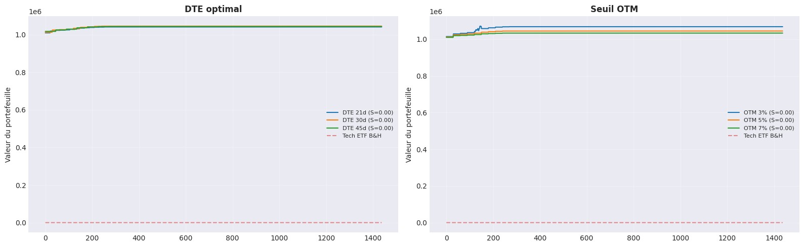
7. Visualisation des résultats

fig, axes = plt.subplots(1, 2, figsize=(16, 5))

# Gauche: DTE comparison
ax = axes[0]
for name, r in dte_results.items():
    ax.plot(r['cum'].values, label=f"DTE {name} (S={r['sharpe']:.2f})", linewidth=1.5)
ax.plot(vgt_values.values, label='Tech ETF B&H', linestyle='--', alpha=0.5)
ax.set_title('DTE optimal', fontsize=12, fontweight='bold')
ax.set_ylabel('Valeur du portefeuille')
ax.legend(fontsize=8)
ax.grid(True, alpha=0.3)

# Droite: OTM comparison
ax = axes[1]
for name, r in otm_results.items():
    ax.plot(r['cum'].values, label=f"OTM {name} (S={r['sharpe']:.2f})", linewidth=1.5)
ax.plot(vgt_values.values, label='Tech ETF B&H', linestyle='--', alpha=0.5)
ax.set_title('Seuil OTM', fontsize=12, fontweight='bold')
ax.set_ylabel('Valeur du portefeuille')
ax.legend(fontsize=8)
ax.grid(True, alpha=0.3)

plt.tight_layout()
plt.savefig('wheel_tech_analysis.png', dpi=150, bbox_inches='tight')
plt.show()
print("Graphique sauvegardé.")

Graphique sauvegardé.

8. Conclusions et recommandations

Résumé

Métrique Meilleure config
DTE (à remplir)
OTM (à remplir)
Sharpe (à remplir)
CAGR (à remplir)

Verdict

Si Sharpe > 1.2: Déployer avec les paramètres optimaux

Points forts Wheel Tech

  • Volatilité élevée: Tech stocks = premiums attractifs
  • Revenu régulier: Ventes d’options génèrent du revenu mensuel
  • Diversification: 5 stocks réduit le risque spécifique
  • Adaptatif: OTM par stock selon sa volatilité

Limitations

  • Assignment risk: Possibilité d’être assigné sur les puts
  • Gestion complexe: 5 stocks = 10 positions d’options à gérer
  • Capital intensif: Nécessite du capital pour les margin requirements

Prochaines étapes

  1. Déployer sur QC cloud avec les paramètres optimaux
  2. Tester avec des stocks moins volatils (plus defensifs)
  3. Optimiser le rolling (avant expiration vs à expiration)
  4. Ajouter un filtre de volatilité (VIX) pour éviter les périodes extrêmes
Retour au sommet