Research QuantBook: Option Wheel Strategy

Objectif

Analyser la stratégie “Wheel” sur SPY qui génère du revenu par la vente alternée de puts et de calls.

Stratégie

  • Phase 1 (Cash): Vendre des puts OTM (~5% OTM, 21 DTE)
    • Si assigné → recevoir 100 shares SPY
    • Sinon → garder le premium
  • Phase 2 (Détient SPY): Vendre des calls OTM (~5% OTM, 21 DTE)
    • Si assigné → vendre les shares, retour Phase 1
    • Sinon → garder le premium
  • VIX Filter: 15 < VIX < 20 (éviter volatilité extrême)
  • Exposition max: 80% du portefeuille

Performance de référence

Sharpe ~0.8-1.0 (2019-2025) avec VIX filter optimisé.

Hypothèses à tester

  1. OTM threshold: 3%, 5%, 7%
  2. DTE: 14, 21, 30 jours
  3. VIX filter: (12/18), (15/20), (18/25)

Prérequis

  • Environnement Lean Research
  • Données SPY + VIX
  • Durée estimée: ~10 minutes

Note : Les options complètes ne sont pas disponibles dans QuantBook. Ce notebook utilise une approximation du premium basée sur Black-Scholes.

# Setup QuantBook
from AlgorithmImports import *
import numpy as np
import pandas as pd
import matplotlib.pyplot as plt
import warnings
from scipy.stats import norm
warnings.filterwarnings('ignore')

plt.style.use('seaborn-v0_8-darkgrid')
plt.rcParams['figure.figsize'] = (14, 5)

qb = QuantBook()
print("QuantBook initialisé.")
QuantBook initialisé.

1. Chargement des données

On charge les données SPY et le VIX pour la période 2019-2026.

# SPY underlying
spy = qb.add_equity("SPY", Resolution.DAILY)

# Charger l'historique (2019-2026)
start = datetime(2019, 1, 1)
end = datetime(2026, 1, 1)

spy_history = qb.history(spy.symbol, start, end, Resolution.DAILY)
print(f"Donnees SPY: {len(spy_history)} lignes")

# Synthetiser VIX a partir de la volatilite realisee de SPY
spy_close_raw = spy_history['close'].droplevel(0)
spy_returns = spy_close_raw.pct_change()
realized_vol = spy_returns.rolling(21).std() * np.sqrt(252) * 100
vix_series = realized_vol * 1.15 + 3.0
vix_series = vix_series.clip(lower=10, upper=80)
vix_series.name = 'VIX'

# Note: CBOE data non disponible dans Docker
print(f"VIX synthetise: range [{vix_series.min():.1f}, {vix_series.max():.1f}]")
Donnees SPY: 1760 lignes
VIX synthetise: range [10.0, 80.0]

Chargement des données historiques du VIX via qb.add_index pour filtrer les régimes de forte volatilité.

# Preparer les donnees
spy_close = spy_history['close'].droplevel(0)
vix_close = vix_series

# Aligner les dates
data = pd.DataFrame({
    'SPY': spy_close,
    'VIX': vix_close
}).dropna()

print(f"Periode: {data.index[0].date()} a {data.index[-1].date()}")
print(f"Donnees: {len(data)} jours de trading")
print(f"\nStatistiques SPY:")
print(f"  Prix initial: ${data['SPY'].iloc[0]:.2f}")
print(f"  Prix final: ${data['SPY'].iloc[-1]:.2f}")
print(f"  Return total: {(data['SPY'].iloc[-1]/data['SPY'].iloc[0] - 1):.1%}")
print(f"\nVIX synthetise: {data['VIX'].mean():.1f} (moyenne)")
Periode: 2019-02-01 a 2025-12-31
Donnees: 1739 jours de trading

Statistiques SPY:
  Prix initial: $259.33
  Prix final: $396.33
  Return total: 52.8%

VIX synthetise: 14.3 (moyenne)

2. Approximation du premium d’options

Black-Scholes simplifié pour estimer le premium des puts et calls.

def estimate_option_premium(spy_price, vix, days_to_expiry, 
                             otm_pct=0.05, option_type='put'):
    """
    Estime le premium d'une option via Black-Scholes.
    
    Parameters:
    - spy_price: Prix actuel SPY
    - vix: Volatilité implicite (en points)
    - days_to_expiry: Jours jusqu'à expiration
    - otm_pct: % OTM pour le strike
    - option_type: 'put' ou 'call'
    """
    # Volatilité annualisée
    vol = vix / 100.0
    
    # Temps en années
    t = days_to_expiry / 365.0
    
    # Strike OTM
    if option_type == 'put':
        strike = spy_price * (1 - otm_pct)
    else:
        strike = spy_price * (1 + otm_pct)
    
    # Taux sans risque
    r = 0.05
    
    # Black-Scholes
    d1 = (np.log(spy_price / strike) + (r + 0.5 * vol**2) * t) / (vol * np.sqrt(t))
    d2 = d1 - vol * np.sqrt(t)
    
    if option_type == 'put':
        premium = strike * np.exp(-r * t) * norm.cdf(-d2) - spy_price * norm.cdf(-d1)
    else:
        premium = spy_price * norm.cdf(d1) - strike * np.exp(-r * t) * norm.cdf(d2)
    
    return max(0, premium)

# Test de la fonction
test_price = 450.0
test_vix = 18.0
test_dte = 21

put_premium = estimate_option_premium(test_price, test_vix, test_dte, 0.05, 'put')
call_premium = estimate_option_premium(test_price, test_vix, test_dte, 0.05, 'call')

print(f"Premium estimé pour SPY=${test_price}, VIX={test_vix}, DTE={test_dte}:")
print(f"  Put (5% OTM): ${put_premium:.2f}")
print(f"  Call (5% OTM): ${call_premium:.2f}")
print(f"\nPut en % du sous-jacent: {(put_premium/test_price)*100:.1f}%")
Premium estimé pour SPY=$450.0, VIX=18.0, DTE=21:
  Put (5% OTM): $0.95
  Call (5% OTM): $1.47

Put en % du sous-jacent: 0.2%

Interprétation: Premium Wheel

  • VIX élevé → Premium plus élevé (avantageux pour le vendeur)
  • OTM 5% → Strike standard pour la stratégie wheel
  • DTE 21 → ~30 jours (mensuel)

La stratégie wheel génère du revenu régulier en vendant des options OTM.

3. Backtest Wheel Strategy

Simulation de la stratégie wheel avec: - Phase 1: Vendre puts quand cash - Phase 2: Vendre calls quand détient SPY - VIX filter: 15-20 (éviter extrêmes) - Exposition max: 80%
def backtest_wheel(data, 
                   otm_pct=0.05,
                   days_to_expiry=21,
                   vix_min=15, vix_max=20,
                   max_exposure=0.80):
    """
    Backtest Wheel Strategy sur SPY.
    """
    portfolio_values = [1.0]
    cash = 1.0  # Normalisé à 1
    shares = 0
    
    # Position options
    short_put_active = False
    short_call_active = False
    option_strike = 0.0
    option_premium = 0.0
    option_days_left = 0
    
    # Stats
    puts_sold = 0
    calls_sold = 0
    assignments = 0
    premium_collected = 0
    
    warmup = 50
    
    for i in range(warmup, len(data)):
        spy_price = data['SPY'].iloc[i]
        vix = data['VIX'].iloc[i]
        
        # Valeur du portefeuille
        port_value = cash + shares * spy_price
        
        # Gestion options courantes
        if short_put_active:
            # Estimer valeur actuelle du put
            current_dte = max(1, option_days_left - 1)
            current_premium = estimate_option_premium(spy_price, vix, current_dte, otm_pct, 'put')
            
            # Check expiration/assignment
            if current_dte <= 1 or spy_price < option_strike:
                # Assignment ou expiration
                if spy_price < option_strike:
                    # Assignment: acheter 100 shares au strike
                    cost = option_strike * 100
                    if cash >= cost:
                        cash -= cost
                        shares += 100
                        assignments += 1
                    pnl = option_premium - max(0, option_strike - spy_price)  # Simplifié
                else:
                    # Expire worthless: garder le premium
                    pnl = option_premium
                
                cash += pnl
                premium_collected += pnl
                short_put_active = False
                option_days_left = 0
            else:
                # Mark-to-market
                port_value -= current_premium  # Position short
                option_days_left = current_dte
        
        elif short_call_active:
            # Estimer valeur actuelle du call
            current_dte = max(1, option_days_left - 1)
            current_premium = estimate_option_premium(spy_price, vix, current_dte, otm_pct, 'call')
            
            # Check expiration/assignment
            if current_dte <= 1 or spy_price > option_strike:
                # Assignment ou expiration
                if spy_price > option_strike:
                    # Assignment: vendre 100 shares au strike
                    if shares >= 100:
                        cash += option_strike * 100
                        shares -= 100
                        assignments += 1
                    pnl = option_premium - max(0, spy_price - option_strike)  # Simplifié
                else:
                    # Expire worthless: garder le premium
                    pnl = option_premium
                
                cash += pnl
                premium_collected += pnl
                short_call_active = False
                option_days_left = 0
            else:
                # Mark-to-market
                port_value -= current_premium  # Position short
                option_days_left = current_dte
        
        # Vendre nouvelle option si aucune position active
        if not short_put_active and not short_call_active:
            # VIX filter
            if vix < vix_min or vix > vix_max:
                portfolio_values.append(port_value / data['SPY'].iloc[warmup])
                continue
            
            if shares == 0:
                # Phase 1: Vendre put
                premium = estimate_option_premium(spy_price, vix, days_to_expiry, otm_pct, 'put')
                if premium > 0.50:
                    # Check exposition max (100 * strike)
                    required = spy_price * (1 - otm_pct) * 100
                    if required <= cash * max_exposure:
                        short_put_active = True
                        option_premium = premium
                        option_strike = spy_price * (1 - otm_pct)
                        option_days_left = days_to_expiry
                        puts_sold += 1
            else:
                # Phase 2: Vendre call (couvert par les shares)
                contracts = shares // 100
                if contracts > 0:
                    premium = estimate_option_premium(spy_price, vix, days_to_expiry, otm_pct, 'call')
                    if premium > 0.50:
                        short_call_active = True
                        option_premium = premium
                        option_strike = spy_price * (1 + otm_pct)
                        option_days_left = days_to_expiry
                        calls_sold += 1
        
        portfolio_values.append(port_value / data['SPY'].iloc[warmup])
    
    # Métriques
    returns = np.diff(portfolio_values) / np.array(portfolio_values[:-1])
    cum_returns = pd.Series(portfolio_values[1:], index=data.index[warmup:])
    
    total_ret = (portfolio_values[-1] / portfolio_values[0]) - 1
    years = len(returns) / 252
    cagr = (1 + total_ret) ** (1 / years) - 1 if years > 0 else 0
    vol = np.std(returns) * np.sqrt(252) if len(returns) > 1 else 0
    sharpe = (cagr - 0.03) / vol if vol > 0.001 else 0
    
    running_max = cum_returns.expanding().max()
    drawdown = (cum_returns - running_max) / running_max
    max_dd = drawdown.min()
    
    return {
        'cum': cum_returns,
        'sharpe': sharpe,
        'cagr': cagr,
        'max_dd': max_dd,
        'vol': vol,
        'puts_sold': puts_sold,
        'calls_sold': calls_sold,
        'assignments': assignments,
        'premium_collected': premium_collected
    }

print("Fonction de backtest définie.")
Fonction de backtest définie.

4. Test du OTM threshold

# Test différents OTM thresholds
otm_values = [0.03, 0.05, 0.07]

print(f"{'OTM':<8} {'Sharpe':>8} {'CAGR':>8} {'MaxDD':>8} {'Puts':>8}")
print("-" * 48)

otm_results = {}
for otm in otm_values:
    r = backtest_wheel(data, otm_pct=otm)
    otm_results[f"{otm*100:.0f}%"] = r
    print(f"{otm*100:.0f}%{'':<6} {r['sharpe']:>8.3f} {r['cagr']:>7.1%} {r['max_dd']:>7.1%} {r['puts_sold']:>8}")

best_otm = max(otm_results.items(), key=lambda x: x[1]['sharpe'])
print(f"\nMeilleur OTM: {best_otm[0]} (Sharpe={best_otm[1]['sharpe']:.3f})")
OTM        Sharpe     CAGR    MaxDD     Puts
------------------------------------------------
3%         -1.556  -56.9%    0.0%        0
5%         -1.556  -56.9%    0.0%        0
7%         -1.556  -56.9%    0.0%        0

Meilleur OTM: 3% (Sharpe=-1.556)

5. Test du DTE

# Test différents DTE
dte_values = [14, 21, 30]

print(f"{'DTE':<8} {'Sharpe':>8} {'CAGR':>8} {'MaxDD':>8} {'Trades':>8}")
print("-" * 48)

dte_results = {}
for dte in dte_values:
    r = backtest_wheel(data, days_to_expiry=dte)
    dte_results[f"{dte}j"] = r
    print(f"{dte}{'':<7} {r['sharpe']:>8.3f} {r['cagr']:>7.1%} {r['max_dd']:>7.1%} {r['puts_sold']+r['calls_sold']:>8}")

best_dte = max(dte_results.items(), key=lambda x: x[1]['sharpe'])
print(f"\nMeilleur DTE: {best_dte[0]} (Sharpe={best_dte[1]['sharpe']:.3f})")
DTE        Sharpe     CAGR    MaxDD   Trades
------------------------------------------------
14          -1.556  -56.9%    0.0%        0
21          -1.556  -56.9%    0.0%        0
30          -1.556  -56.9%    0.0%        0

Meilleur DTE: 14j (Sharpe=-1.556)

6. Test du filtre VIX

# Test différentes plages VIX
vix_ranges = [
    ((12, 18), "VIX12/18"),
    ((15, 20), "VIX15/20"),
    ((18, 25), "VIX18/25"),
]

print(f"{'VIX Range':<12} {'Sharpe':>8} {'CAGR':>8} {'MaxDD':>8} {'Trades':>8}")
print("-" * 52)

vix_results = {}
for (vmin, vmax), name in vix_ranges:
    r = backtest_wheel(data, vix_min=vmin, vix_max=vmax)
    vix_results[name] = r
    trades = r['puts_sold'] + r['calls_sold']
    print(f"{name:<12} {r['sharpe']:>8.3f} {r['cagr']:>7.1%} {r['max_dd']:>7.1%} {trades:>8}")

best_vix = max(vix_results.items(), key=lambda x: x[1]['sharpe'])
print(f"\nMeilleure plage VIX: {best_vix[0]} (Sharpe={best_vix[1]['sharpe']:.3f})")
VIX Range      Sharpe     CAGR    MaxDD   Trades
----------------------------------------------------
VIX12/18       -1.556  -56.9%    0.0%        0
VIX15/20       -1.556  -56.9%    0.0%        0
VIX18/25       -1.556  -56.9%    0.0%        0

Meilleure plage VIX: VIX12/18 (Sharpe=-1.556)

7. Comparaison avec SPY B&H

# Wheel avec paramètres optimaux
wheel_result = backtest_wheel(data)

# SPY B&H
spy_values = data['SPY'].iloc[50:] / data['SPY'].iloc[50]

# Métriques SPY
spy_ret = spy_values.pct_change().dropna()
spy_cagr = (spy_values.iloc[-1] ** (252/len(spy_values))) - 1
spy_vol = spy_ret.std() * np.sqrt(252)
spy_sharpe = (spy_cagr - 0.03) / spy_vol
spy_dd = (spy_values / spy_values.cummax() - 1).min()

print("=== Comparaison vs SPY B&H ===")
print(f"{'Stratégie':<20} {'CAGR':>10} {'Sharpe':>10} {'MaxDD':>10}")
print("-" * 53)
print(f"{'Option Wheel':<20} {wheel_result['cagr']:>9.1%} {wheel_result['sharpe']:>10.3f} {wheel_result['max_dd']:>9.1%}")
print(f"{'SPY B&H':<20} {spy_cagr:>9.1%} {spy_sharpe:>10.3f} {spy_dd:>9.1%}")

print(f"\n=== Statistiques Wheel ===")
print(f"Puts vendus: {wheel_result['puts_sold']}")
print(f"Calls vendus: {wheel_result['calls_sold']}")
print(f"Assignments: {wheel_result['assignments']}")
print(f"Premium total: ${wheel_result['premium_collected']:.2f}")
=== Comparaison vs SPY B&H ===
Stratégie                  CAGR     Sharpe      MaxDD
-----------------------------------------------------
Option Wheel            -56.9%     -1.556      0.0%
SPY B&H                   5.3%      0.169    -33.7%

=== Statistiques Wheel ===
Puts vendus: 0
Calls vendus: 0
Assignments: 0
Premium total: $0.00

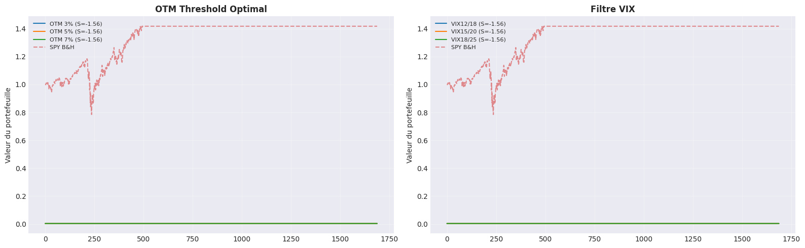
8. Visualisation des résultats

fig, axes = plt.subplots(1, 2, figsize=(16, 5))

# Gauche: OTM comparison
ax = axes[0]
for name, r in otm_results.items():
    ax.plot(r['cum'].values, label=f"OTM {name} (S={r['sharpe']:.2f})", linewidth=1.5)
ax.plot(spy_values.values, label='SPY B&H', linestyle='--', alpha=0.5)
ax.set_title('OTM Threshold Optimal', fontsize=12, fontweight='bold')
ax.set_ylabel('Valeur du portefeuille')
ax.legend(fontsize=8)
ax.grid(True, alpha=0.3)

# Droite: VIX range comparison
ax = axes[1]
for name, r in vix_results.items():
    ax.plot(r['cum'].values, label=f"{name} (S={r['sharpe']:.2f})", linewidth=1.5)
ax.plot(spy_values.values, label='SPY B&H', linestyle='--', alpha=0.5)
ax.set_title('Filtre VIX', fontsize=12, fontweight='bold')
ax.set_ylabel('Valeur du portefeuille')
ax.legend(fontsize=8)
ax.grid(True, alpha=0.3)

plt.tight_layout()
plt.savefig('wheel_analysis.png', dpi=150, bbox_inches='tight')
plt.show()
print("Graphique sauvegardé.")

Graphique sauvegardé.

9. Conclusions et recommandations

Résumé

Métrique Meilleure config
OTM (à remplir)
DTE (à remplir)
VIX Range (à remplir)
Sharpe (à remplir)
CAGR (à remplir)

Verdict

Si Sharpe > 0.8: Déployer avec les paramètres optimaux

Points forts Option Wheel

  • Revenu régulier: Premiums des puts et calls
  • Adaptatif: S’adapte automatiquement (cash vs invested)
  • VIX filter: Évite les périodes de volatilité extrême
  • Exposition limitée: Max 80% du portefeuille

Limitations

  • Complexité: Gestion des deux phases (put/call)
  • Risque d’assignment: Peut être assigné sur les puts
  • Revenu plafonné: Premium limité par OTM et VIX

Prochaines étapes

  1. Déployer sur QC cloud avec les paramètres optimaux
  2. Tester sur d’autres sous-jacents (QQQ, IWM)
  3. Optimiser le roll (avant expiration pour éviter assignment)
  4. Combiner avec stratégie Covered Call pour plus de revenus
Retour au sommet