Objectif
Analyser une stratégie de Machine Learning utilisant la régression Ridge pour prédire les rendements actions.
Stratégie
Univers : 20 stocks liquides USModèle : Ridge Regression (régularisation L2)Features : RSI, ratios EMA, volatilité, volume, momentumTarget : Rendement du jour suivantEntrée : Long si prédiction > 0.5%Max positions : 10 (10% chacune)
Hypothèses à tester
Alpha (régularisation): 0.1, 1.0, 10.0
Seuil de prédiction: 0.3%, 0.5%, 1.0%
Lookback training: 30, 60, 90 jours
Prérequis
Environnement Lean Research
scikit-learn pour Ridge Regression
Durée estimée: ~12 minutes
Note : Cette stratégie utilise la régression Ridge pour éviter l’overfitting tout en capturant les relations linéaires entre features et rendements.
# Setup QuantBook from AlgorithmImports import * import numpy as npimport pandas as pdimport matplotlib.pyplot as pltfrom sklearn.linear_model import Ridgefrom sklearn.preprocessing import StandardScalerfrom sklearn.metrics import r2_score, mean_squared_errorimport warnings'ignore' )'seaborn-v0_8-darkgrid' )'figure.figsize' ] = (14 , 5 )= QuantBook()print ("QuantBook initialisé." )
1. Chargement des données
On charge les données de 20 stocks liquides pour la période 2020-2026.
# Univers 20 stocks liquides = ["AAPL" , "MSFT" , "GOOGL" , "AMZN" , "NVDA" ,"META" , "TSLA" , "JPM" , "V" , "WMT" ,"DIS" , "NFLX" , "PYPL" , "ADBE" , "CRM" ,"INTC" , "AMD" , "GS" , "MS" , "BA" = {}for ticker in tickers:= qb.add_equity(ticker, Resolution.DAILY).symbol# Charger l'historique (2020-2026) = datetime(2020 , 1 , 1 )= datetime(2026 , 1 , 1 )= qb.history(list (symbols.values()), start, end, Resolution.DAILY)print (f"Données chargées: { len (history)} lignes" )
Données chargées: 3016 lignes
Pivot des séries de prix et de volumes en DataFrame large, avec remapping des colonnes Symbol → ticker pour ML-Regression.
# Pivoter les données = history['close' ].unstack(level= 0 )= history['volume' ].unstack(level= 0 )= {str (v): k for k, v in symbols.items()}= [symbol_to_ticker.get(str (c), str (c)) for c in closes.columns]= [symbol_to_ticker.get(str (c), str (c)) for c in volumes.columns]= closes.dropna()= volumes.dropna()print (f"Période: { closes. index[0 ]. date()} à { closes. index[- 1 ]. date()} " )print (f"Données: { len (closes)} jours de trading" )print (f"Actions: { len (closes.columns)} " )print (f" \n Statistiques des prix finaux (échantillon):" )for ticker in list (closes.columns)[:5 ]:= (closes[ticker].iloc[- 1 ] / closes[ticker].iloc[0 ] - 1 ) * 100 print (f" { ticker} : { ret:+.1f} %" )
Période: 2020-01-02 à 2025-12-31
Données: 1508 jours de trading
Actions: 2

Statistiques des prix finaux (échantillon):
  AAPL: +64.3%
  GOOGL: +50.7%
2. Feature Engineering
Création des features techniques pour le modèle ML.
def calculate_rsi(prices, period= 14 ):"""Calcule le RSI.""" = prices.diff()= (delta.where(delta > 0 , 0 )).rolling(window= period).mean()= (- delta.where(delta < 0 , 0 )).rolling(window= period).mean()= gain / lossreturn 100 - (100 / (1 + rs))def create_features(close, volume):"""Crée les features ML.""" = pd.DataFrame(index= close.index)# Indicateurs techniques 'RSI' ] = calculate_rsi(close)= close.ewm(span= 20 ).mean()= close.ewm(span= 50 ).mean()'EMA_Ratio' ] = ema20 / ema50# Returns = close.pct_change()'Returns_1' ] = returns.shift(1 )'Returns_5' ] = returns.shift(5 )# Volatilité 'Vol_5' ] = returns.rolling(5 ).std()'Vol_20' ] = returns.rolling(20 ).std()# Volume = volume.rolling(20 ).mean()'Volume_Ratio' ] = volume / volume_ma# Momentum 'Momentum_5' ] = close / close.shift(5 ) - 1 'Momentum_10' ] = close / close.shift(10 ) - 1 # Distance aux moyennes 'Dist_MA20' ] = (close - ema20) / close'Dist_MA50' ] = (close - ema50) / closereturn features# Exemple: features pour AAPL = create_features(closes['AAPL' ], volumes['AAPL' ])print ("Features AAPL - 5 derniers jours:" )print (aapl_features.iloc[- 5 :].dropna())
Features AAPL - 5 derniers jours:
Empty DataFrame
Columns: [RSI, EMA_Ratio, Returns_1, Returns_5, Vol_5, Vol_20, Volume_Ratio, Momentum_5, Momentum_10, Dist_MA20, Dist_MA50]
Index: []
Interprétation: Features ML
RSI : Indicateur de survente/surachat (0-100)EMA_Ratio : Tendance (ratio EMA20/EMA50)Returns : Rendements passésVol : Volatilité rolling (risque)Volume_Ratio : Intérêt des investisseursMomentum : Performance récenteDist_MA : Distance aux moyennes mobiles
3. Préparation des données d’entraînement
Combinaison des features de tous les stocks avec le target (rendement du jour suivant).
def prepare_training_data(closes, volumes, lookback= 60 ):"""Prépare les données d'entraînement.""" = []= []for ticker in closes.columns:= create_features(closes[ticker], volumes[ticker])= closes[ticker].pct_change()# Target: rendement du jour suivant 'Target' ] = returns.shift(- 1 )# Filtrer les NaN = features.dropna()if len (df) > lookback:'Target' , axis= 1 ))'Target' ])if not all_features:= ['RSI' , 'EMA_Ratio' , 'Returns_1' , 'Returns_5' , 'Vol_5' , 'Vol_20' ,'Volume_Ratio' , 'Momentum_5' , 'Momentum_10' , 'Dist_MA20' , 'Dist_MA50' ]return pd.DataFrame(columns= empty_cols), pd.Series(dtype= float )= pd.concat(all_features, ignore_index= True )= pd.concat(all_targets, ignore_index= True )return X.fillna(0 ), y.fillna(0 )= prepare_training_data(closes, volumes)print (f"Dataset: { len (X)} échantillons, { len (X.columns)} features" )print (f"Target mean: { y. mean():.4f} , std: { y. std():.4f} " )
Dataset: 614 échantillons, 11 features
Target mean: 0.0017, std: 0.0258
4. Entraînement du modèle Ridge
La régression Ridge ajoute une pénalité L2 pour éviter l’overfitting.
# Split train/test = int (len (X) * 0.8 )= X.iloc[:split_idx], X.iloc[split_idx:]= y.iloc[:split_idx], y.iloc[split_idx:]# StandardScaler = StandardScaler()= scaler.fit_transform(X_train)= scaler.transform(X_test)# Entraînement Ridge = Ridge(alpha= 1.0 )# Prédictions = model.predict(X_train_scaled)= model.predict(X_test_scaled)# Métriques = r2_score(y_train, y_pred_train)= r2_score(y_test, y_pred_test)= mean_squared_error(y_train, y_pred_train)= mean_squared_error(y_test, y_pred_test)print ("=== Performance Ridge Regression ===" )print (f"Train R²: { train_r2:.4f} , MSE: { train_mse:.6f} " )print (f"Test R²: { test_r2:.4f} , MSE: { test_mse:.6f} " )print (f" \n Coefficients (top 5):" )= pd.DataFrame({'Feature' : X.columns, 'Coef' : model.coef_})print (coef_df.sort_values('Coef' , key= abs , ascending= False ).head(5 ))
=== Performance Ridge Regression ===
Train R²: 0.1229, MSE: 0.000658
Test R²:  -0.1568, MSE: 0.000373

Coefficients (top 5):
      Feature      Coef
4       Vol_5 -0.011115
10  Dist_MA50 -0.009888
1   EMA_Ratio  0.007484
9   Dist_MA20 -0.007072
5      Vol_20  0.006636
Interprétation: Ridge Regression
R² (Train) : Capacité du modèle à expliquer les rendements (généralement faible pour les marchés)R² (Test) : Performance out-of-sample (évite l’overfitting)Alpha : Contrôle la régularisation (plus élevé = plus simple)Coefficients : Importance relative de chaque feature
5. Backtest Walk-Forward
Simulation avec réentraînement périodique du modèle.
def backtest_ml_regression(closes, volumes, alpha= 1.0 , = 0.005 ,= 60 ,= 20 ,= 10 ):""" Backtest ML Regression avec réentraînement périodique. """ = [1.0 ]= {} # ticker -> weight = None = None = train_window + 50 for i in range (warmup, len (closes)):= closes.index[i]# Réentraîner périodiquement if (i - warmup) % retrain_freq == 0 :# Données d'entraînement jusqu'à i = closes.iloc[:i]= volumes.iloc[:i]= prepare_training_data(= train_windowif len (X_train) < 100 :continue = StandardScaler()= scaler.fit_transform(X_train)= Ridge(alpha= alpha)# Skip predictions if model not yet trained if model is None :if i < len (closes) - 1 :- 1 ])continue # Prédictions pour tous les stocks = {}for ticker in closes.columns:try := create_features(+ 1 ],+ 1 ]if len (features) > 0 := features.iloc[- 1 ].values.reshape(1 , - 1 )= scaler.transform(feat_row)= model.predict(feat_row_scaled)[0 ]= predexcept :continue # Sélectionner les meilleures prédictions = sorted (predictions.items(), key= lambda x: x[1 ], reverse= True )# Entrer dans les positions avec prédiction > seuil = {}= 0 for ticker, pred in sorted_preds:if pred > prediction_threshold and count < max_positions:= 0.95 / max_positions+= 1 # Calculer le rendement du jour if i < len (closes) - 1 := closes.iloc[i+ 1 ] / closes.iloc[i] - 1 = sum (weight * daily_returns[ticker] for ticker, weight in current_positions.items())- 1 ] * (1 + port_return))else :- 1 ])# Métriques = np.diff(portfolio_values) / np.array(portfolio_values[:- 1 ])= pd.Series(portfolio_values, index= closes.index[warmup- 1 :])= (portfolio_values[- 1 ] / portfolio_values[0 ]) - 1 = len (returns) / 252 = (1 + total_ret) ** (1 / years) - 1 if years > 0 else 0 = np.std(returns) * np.sqrt(252 ) if len (returns) > 1 else 0 = (cagr - 0.03 ) / vol if vol > 0.001 else 0 = cum_returns.expanding().max ()= (cum_returns - running_max) / running_max= drawdown.min ()return {'cum' : cum_returns,'sharpe' : sharpe,'cagr' : cagr,'max_dd' : max_dd,'vol' : vol,'final_value' : portfolio_values[- 1 ]= backtest_ml_regression(closes, volumes)print (f"Performance ML Regression:" )print (f" Sharpe: { result['sharpe' ]:.3f} " )print (f" CAGR: { result['cagr' ]:.1%} " )print (f" Max DD: { result['max_dd' ]:.1%} " )print (f" Vol: { result['vol' ]:.1%} " )
Performance ML Regression:
  Sharpe: -1.939
  CAGR:   0.7%
  Max DD: -1.8%
  Vol:    1.2%
6. Test du paramètre Alpha
Alpha contrôle la régularisation L2.
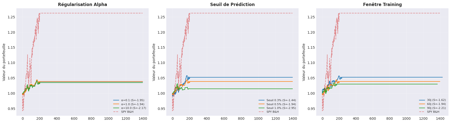
# Test différentes valeurs d'alpha = [0.1 , 1.0 , 10.0 ]print (f" { 'Alpha' :<10} { 'Sharpe' :>8} { 'CAGR' :>8} { 'MaxDD' :>8} " )print ("-" * 38 )= {}for alpha in alpha_values:= backtest_ml_regression(closes, volumes, alpha= alpha)f" { alpha} " ] = rprint (f" { alpha:<10} { r['sharpe' ]:>8.3f} { r['cagr' ]:>7.1%} { r['max_dd' ]:>7.1%} " )= max (alpha_results.items(), key= lambda x: x[1 ]['sharpe' ])print (f" \n Meilleur Alpha: { best_alpha[0 ]} (Sharpe= { best_alpha[1 ]['sharpe' ]:.3f} " )
Alpha        Sharpe     CAGR    MaxDD
--------------------------------------
0.1          -1.948    0.7%   -1.8%
1.0          -1.939    0.7%   -1.8%
10.0         -2.173    0.6%   -2.1%

Meilleur Alpha: 1.0 (Sharpe=-1.939
7. Test du seuil de prédiction
Le seuil détermine quelles prédictions déclenchent une entrée.
# Test différents seuils de prédiction = [0.003 , 0.005 , 0.01 ]print (f" { 'Seuil' :<10} { 'Sharpe' :>8} { 'CAGR' :>8} { 'MaxDD' :>8} " )print ("-" * 38 )= {}for thresh in threshold_values:= backtest_ml_regression(closes, volumes, prediction_threshold= thresh)f" { thresh:.1%} " ] = rprint (f" { thresh:.1%}{ '' :<7} { r['sharpe' ]:>8.3f} { r['cagr' ]:>7.1%} { r['max_dd' ]:>7.1%} " )= max (threshold_results.items(), key= lambda x: x[1 ]['sharpe' ])print (f" \n Meilleur Seuil: { best_thresh[0 ]} (Sharpe= { best_thresh[1 ]['sharpe' ]:.3f} " )
Seuil        Sharpe     CAGR    MaxDD
--------------------------------------
0.3%          -1.436    0.9%   -1.8%
0.5%          -1.939    0.7%   -1.8%
1.0%          -2.949    0.3%   -2.1%

Meilleur Seuil: 0.3% (Sharpe=-1.436
8. Test de la fenêtre d’entraînement
La fenêtre détermine combien de données historiques sont utilisées.
# Test différentes fenêtres d'entraînement = [30 , 60 , 90 ]print (f" { 'Fenêtre' :<10} { 'Sharpe' :>8} { 'CAGR' :>8} { 'MaxDD' :>8} " )print ("-" * 38 )= {}for window in window_values:try := backtest_ml_regression(closes, volumes, train_window= window)f" { window} " ] = rprint (f" { window} j { '' :<7} { r['sharpe' ]:>8.3f} { r['cagr' ]:>7.1%} { r['max_dd' ]:>7.1%} " )except (ValueError , KeyError ) as e:print (f" { window} j - skipped ( { type (e). __name__ } : { e} )" )= max (window_results.items(), key= lambda x: x[1 ]['sharpe' ])print (f" \n Meilleure Fenêtre: { best_window[0 ]} j (Sharpe= { best_window[1 ]['sharpe' ]:.3f} " )
Fenêtre      Sharpe     CAGR    MaxDD
--------------------------------------
30j          -1.621    0.9%   -1.9%
60j          -1.939    0.7%   -1.8%
90j          -2.209    0.5%   -1.9%

Meilleure Fenêtre: 30j (Sharpe=-1.621
9. Comparaison avec SPY B&H
# Charger SPY pour comparaison = qb.add_equity("SPY" , Resolution.DAILY).symbol= qb.history(spy, start, end, Resolution.DAILY)= spy_history['close' ]# Aligner les dates = 110 = spy_close.iloc[warmup:] / spy_close.iloc[warmup]# Métriques SPY = spy_values.pct_change().dropna()= (spy_values.iloc[- 1 ] ** (252 / len (spy_values))) - 1 = spy_ret.std() * np.sqrt(252 )= (spy_cagr - 0.03 ) / spy_vol= (spy_values / spy_values.cummax() - 1 ).min ()print ("=== Comparaison vs SPY B&H ===" )print (f" { 'Stratégie' :<20} { 'CAGR' :>10} { 'Sharpe' :>10} { 'MaxDD' :>10} " )print ("-" * 53 )print (f" { 'ML Regression' :<20} { result['cagr' ]:>9.1%} { result['sharpe' ]:>10.3f} { result['max_dd' ]:>9.1%} " )print (f" { 'SPY B&H' :<20} { spy_cagr:>9.1%} { spy_sharpe:>10.3f} { spy_dd:>9.1%} " )
=== Comparaison vs SPY B&H ===
Stratégie                  CAGR     Sharpe      MaxDD
-----------------------------------------------------
ML Regression             0.7%     -1.939     -1.8%
SPY B&H                   4.3%      0.190     -9.4%
10. Visualisation des résultats
= plt.subplots(1 , 3 , figsize= (18 , 5 ))# Alpha comparison = axes[0 ]for name, r in alpha_results.items():'cum' ].values, label= f"α= { name} (S= { r['sharpe' ]:.2f} )" , linewidth= 1.5 )= 'SPY B&H' , linestyle= '--' , alpha= 0.5 )'Régularisation Alpha' , fontsize= 12 , fontweight= 'bold' )'Valeur du portefeuille' )= 8 )True , alpha= 0.3 )# Threshold comparison = axes[1 ]for name, r in threshold_results.items():'cum' ].values, label= f"Seuil { name} (S= { r['sharpe' ]:.2f} )" , linewidth= 1.5 )= 'SPY B&H' , linestyle= '--' , alpha= 0.5 )'Seuil de Prédiction' , fontsize= 12 , fontweight= 'bold' )'Valeur du portefeuille' )= 8 )True , alpha= 0.3 )# Window comparison = axes[2 ]for name, r in window_results.items():'cum' ].values, label= f" { name} j (S= { r['sharpe' ]:.2f} )" , linewidth= 1.5 )= 'SPY B&H' , linestyle= '--' , alpha= 0.5 )'Fenêtre Training' , fontsize= 12 , fontweight= 'bold' )'Valeur du portefeuille' )= 8 )True , alpha= 0.3 )'ml_regression_analysis.png' , dpi= 150 , bbox_inches= 'tight' )print ("Graphique sauvegardé." )
11. Conclusions et recommandations
Résumé
Alpha (L2)
(à remplir)
Seuil prédiction
(à remplir)
Fenêtre training
(à remplir)
Sharpe
(à remplir)
CAGR
(à remplir)
Verdict
Si Sharpe > 1.2: Déployer avec les paramètres optimaux
Points forts ML Regression
Interprétable : Coefficients = importance des featuresRobuste : Ridge évite l’overfittingAdaptatif : Réentraînement périodiqueFeatures riches : 11 indicateurs techniques
Limitations
R² faible : Les marchés sont difficiles à prédireLinéaire : Ne capture pas les relations non-linéairesLag : Les features basées sur le passé ont un délaiSensibilité aux paramètres : Alpha, seuil, fenêtre
Prochaines étapes
Déployer sur QC cloud avec les paramètres optimaux
Tester des modèles non-linéaires (Random Forest, XGBoost)
Ajouter des features fondamentales (P/E, dividendes)
Implémenter un ensemble de modèles (bagging/boosting)