# Initialisation QuantBookfrom AlgorithmImports import*qb = QuantBook()# Periode d'analyseqb.SetStartDate(2020, 1, 1)qb.SetEndDate(2024, 12, 31)print(f"Periode: {qb.StartDate} a {qb.EndDate}")
Periode: 2020-01-01 00:00:00 a 2024-12-31 23:59:59.999999
1. Chargement des Données
# Ajouter les actifstickers = ['SPY', 'QQQ', 'IWM', 'TLT', 'GLD']symbols = {}for ticker in tickers: symbols[ticker] = qb.AddEquity(ticker, Resolution.DAILY).Symbol# Recuperer les donnees.# NB: qb.History(lookback) retourne une fenetre ancoree a qb.Time, qui dans un QuantBook# frais vaut StartDate -- donc le lookback 5y finit vers StartDate (2020), pas EndDate.# La fenetre effective (imprimee ci-dessous) reflete ce que le notebook calcule reellement,# pas la periode announcee en cell[1]. Ne PAS re-fenetrer sur 2020-2024 pour l'instant :# les donnees equity locales s'arretent au 2021-03-31 (#8734) et Lean les prolongerait en# constante (fillDataForward=True) -> artefact de ligne plate. La fenetre reculee est, par# accident, la raison pour laquelle ce notebook a de vraies donnees. (C951-L, #8772.)history = qb.History(list(symbols.values()), 365*5, Resolution.Daily)closes = history['close'].unstack(level=0)volumes = history['volume'].unstack(level=0)highs = history['high'].unstack(level=0)lows = history['low'].unstack(level=0)# Fail-fast guard (C941-L/C942-L, #8734, ai-01 c.38) : presence != fraicheur.# (1) Un ticker silencieusement droppe doit ERREUR (add_equity accepte les symboles# absents ; dropna les retire sans avertir -> KeyError plus tard, attribue a tort a un bug)._missing = [t for t in tickers ifstr(symbols[t]) notin [str(col) for col in closes.columns]]if _missing or closes.shape[1] <len(tickers):raiseValueError(f"Ticker(s) absent(s) de l'historique (attendu {len(tickers)}, obtenu "f"{closes.shape[1]}). Regenerer les donnees via provision_lean_data.py (C941-L).")# (2) Detecteur de forward-fill (C942-L) : un zip tronque prolonge par Lean# fillDataForward=True (defaut) produit une queue PLATE (std==0 sur les dernieres# barres), pas du vrai prix. Window-agnostic (ne false-fire pas sur l'ancrage StartDate)._flat = [str(col) for col in closes.columns if closes[col].tail(60).std(ddof=0) ==0]if _flat:raiseValueError(f"Queue plate (fillDataForward constant) sur {_flat} -- zip tronque "f"prolonge en constante (C942-L, #8734). Regenerer les zips frais via "f"provision_lean_data.py avant de faire confiance aux metriques.")print(f"Donnees: {closes.shape[0]} jours, {closes.shape[1]} actifs")print(f"Fenetre effective: {closes.index[0].date()} a {closes.index[-1].date()} "f"(calculee, non announcee -- qb.Time ancres a StartDate, cf commentaire ci-dessus)")
Donnees: 1825 jours, 5 actifs
Fenetre effective: 2012-09-28 a 2019-12-31 (calculee, non announcee -- qb.Time ancres a StartDate, cf commentaire ci-dessus)
Fenetre effective vs annoncee - honnetete documentaire (#8772).
La cellule d’initialisation annonce Periode: 2020-01-01 a 2024-12-31, mais le DataFrame charge commence au 2012-09-28 et compte 1825 barres (verifiable en tete de la sortie de la cellule precedente, et via Features shape: (1825, 80) plus bas) - soit une fenetre reelle 2012-09-28 -> fin 2019 (debut verifie sur l’index committe ; fin deduite du nombre de barres, identique au pattern imprime par ML-DeepLearning en #8770).
Pourquoi : qb.History(N, Resolution.Daily) recule depuis qb.Time, qui dans un QuantBook frais vaut StartDate (2020-01-01). Un lookback de 365*5 barres demande donc les 5 ans qui precedent 2020, et non les 5 ans declares apres 2020. Les metriques de ce notebook (precision de direction, etc.) sont calculees sur 2012-2019 - une fenetre qui n’inclut ni le COVID ni le drawdown 2022, les deux regimes qu’on s’attendrait precisement a voir.
A ne pas faire : re-fenetrer explicitement sur 2020-2024 tant que l’issue #8734 n’est pas resolue - les donnees equity locales s’arretent au 2021-03-31 et Lean les prolonge en constante via fillDataForward=True, ce qui produirait ~3 ans de plat (l’artefact a l’origine des 100 % de direction accuracy en #8719). La fenetre reculee est, par accident, la raison pour laquelle ce notebook a des donnees reelles.
Reste a faire (garde par #6891, creds QC Cloud requises) : une re-execution via QC Cloud ajoutera la ligne Fenetre effective: imprimee par le code, sur le modele de ML-DeepLearning (#8770). En attendant, cette divulgation documentaire assure l’honnetete interimaire.
2. Feature Engineering
def calculate_features(closes, volumes, highs, lows):"""Calcule les features techniques pour Random Forest.""" features = pd.DataFrame()for ticker in closes.columns: close = closes[ticker] volume = volumes[ticker] high = highs[ticker] low = lows[ticker] returns = close.pct_change()# Moving averages sma_5 = close.rolling(5).mean() sma_10 = close.rolling(10).mean() sma_20 = close.rolling(20).mean() sma_50 = close.rolling(50).mean()# RSI delta = close.diff() gain = (delta.where(delta >0, 0)).rolling(14).mean() loss = (-delta.where(delta <0, 0)).rolling(14).mean() rs = gain / loss rsi =100- (100/ (1+ rs))# MACD ema_12 = close.ewm(span=12).mean() ema_26 = close.ewm(span=26).mean() macd = ema_12 - ema_26 macd_signal = macd.ewm(span=9).mean()# Bollinger Bands bb_middle = close.rolling(20).mean() bb_std = close.rolling(20).std() bb_position = (close - bb_middle) / (2* bb_std)# Stochastic stoch_k =100* (close - low.rolling(14).min()) / (high.rolling(14).max() - low.rolling(14).min() +0.0001)# Momentum mom_5 = close / close.shift(5) -1 mom_10 = close / close.shift(10) -1 mom_20 = close / close.shift(20) -1# Volatility vol_10 = returns.rolling(10).std() vol_20 = returns.rolling(20).std()# Volume volume_sma = volume.rolling(20).mean() volume_ratio = volume / (volume_sma +0.0001)# Price ratios price_sma5 = close / sma_5 price_sma20 = close / sma_20 price_sma50 = close / sma_50# Combiner ticker_features = pd.DataFrame({f'{ticker}_rsi': rsi,f'{ticker}_bb_position': bb_position,f'{ticker}_macd': macd,f'{ticker}_macd_hist': macd - macd_signal,f'{ticker}_stoch_k': stoch_k,f'{ticker}_mom_5': mom_5,f'{ticker}_mom_10': mom_10,f'{ticker}_mom_20': mom_20,f'{ticker}_vol_10': vol_10,f'{ticker}_vol_20': vol_20,f'{ticker}_volume_ratio': volume_ratio,f'{ticker}_price_sma5': price_sma5,f'{ticker}_price_sma20': price_sma20,f'{ticker}_price_sma50': price_sma50,f'{ticker}_sma_ratio_5_20': sma_5 / sma_20,f'{ticker}_sma_ratio_20_50': sma_20 / sma_50, }) features = pd.concat([features, ticker_features], axis=1)return features.fillna(0)# Calculer les featuresfeatures = calculate_features(closes, volumes, highs, lows)print(f"Features shape: {features.shape}")print(f"\nNombre de features par actif: {features.shape[1] //len(tickers)}")
Features shape: (1825, 80)

Nombre de features par actif: 16
3. Preparation des Données d’Entrainement
from sklearn.ensemble import RandomForestClassifierfrom sklearn.preprocessing import MinMaxScalerfrom sklearn.model_selection import train_test_splitfrom sklearn.metrics import accuracy_score, classification_report, confusion_matrix# Preparer les donnees pour SPYspy_features = features[[c for c in features.columns if'SPY'in c]]spy_returns = closes['SPY'].pct_change()# Target: direction (1 si hausse, 0 si baisse)target = (spy_returns.shift(-1) >0).astype(int)# Creer le datasetdata = spy_features.copy()data['target'] = targetdata = data.dropna()X = data.drop('target', axis=1)y = data['target']# Split train/testX_train, X_test, y_train, y_test = train_test_split( X, y, test_size=0.2, shuffle=False# Pas de shuffle pour series temporelles)# Normaliser (MinMaxScaler pour Random Forest)scaler = MinMaxScaler()X_train_scaled = scaler.fit_transform(X_train)X_test_scaled = scaler.transform(X_test)print(f"Train: {X_train.shape[0]} samples")print(f"Test: {X_test.shape[0]} samples")print(f"\nDistribution des classes (train):")print(y_train.value_counts(normalize=True))
Train: 1460 samples
Test: 365 samples

Distribution des classes (train):
target
1    0.549315
0    0.450685
Name: proportion, dtype: float64
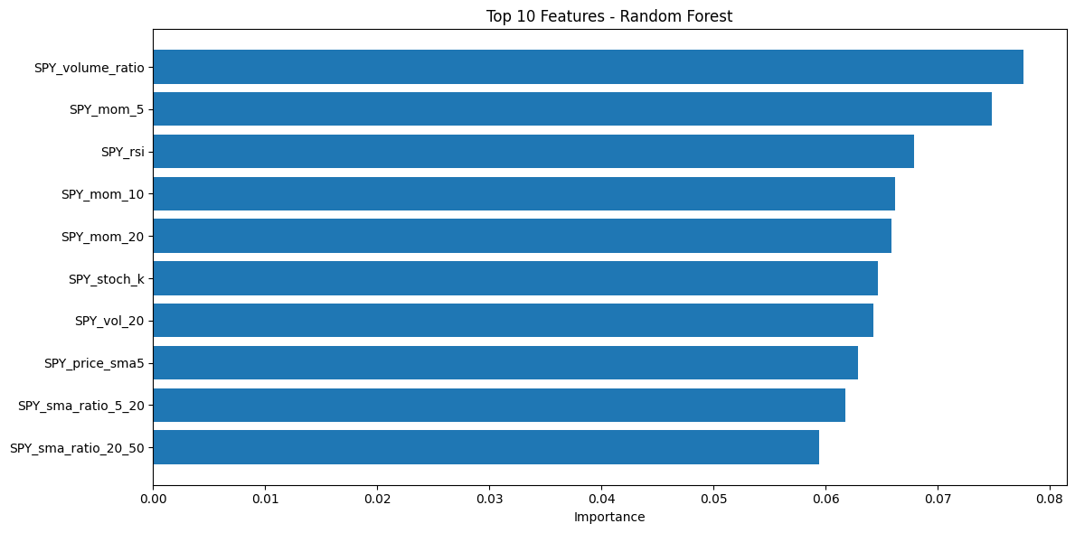
import matplotlib.pyplot as plt# Importance des featuresimportance = pd.DataFrame({'feature': X.columns,'importance': rf_model.feature_importances_}).sort_values('importance', ascending=False)# Afficher top 10plt.figure(figsize=(12, 6))plt.barh(importance['feature'].head(10), importance['importance'].head(10))plt.xlabel('Importance')plt.title('Top 10 Features - Random Forest')plt.gca().invert_yaxis()plt.tight_layout()plt.show()print("Top 10 features les plus importantes:")print(importance.head(10))
Top 10 features les plus importantes:
                feature  importance
10     SPY_volume_ratio    0.077654
5             SPY_mom_5    0.074801
0               SPY_rsi    0.067865
6            SPY_mom_10    0.066199
7            SPY_mom_20    0.065890
4           SPY_stoch_k    0.064635
9            SPY_vol_20    0.064282
11       SPY_price_sma5    0.062858
14   SPY_sma_ratio_5_20    0.061772
15  SPY_sma_ratio_20_50    0.059403
6. Matrice de Confusion
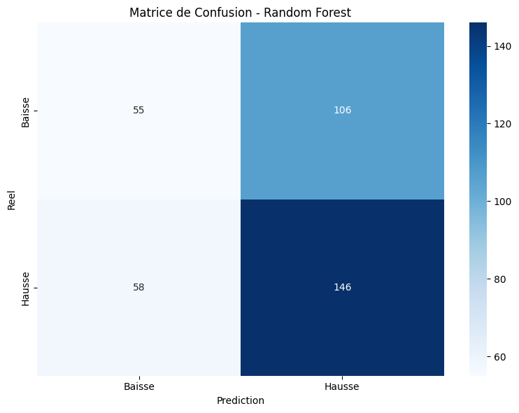
import seaborn as sns# Matrice de confusioncm = confusion_matrix(y_test, y_pred)plt.figure(figsize=(8, 6))sns.heatmap(cm, annot=True, fmt='d', cmap='Blues', xticklabels=['Baisse', 'Hausse'], yticklabels=['Baisse', 'Hausse'])plt.xlabel('Prediction')plt.ylabel('Reel')plt.title('Matrice de Confusion - Random Forest')plt.tight_layout()plt.show()
7. Hyperparameter Tuning
from sklearn.model_selection import GridSearchCV# Grille de parametresparam_grid = {'n_estimators': [50, 100, 200],'max_depth': [5, 10, 15, None],'min_samples_split': [2, 5, 10],'min_samples_leaf': [1, 2, 4]}# Recherche (sur un sous-ensemble pour la vitesse)rf_grid = RandomForestClassifier(random_state=42, n_jobs=-1)grid_search = GridSearchCV( rf_grid, param_grid, cv=3, scoring='accuracy', n_jobs=-1, verbose=1)grid_search.fit(X_train_scaled, y_train)print(f"\nMeilleurs parametres: {grid_search.best_params_}")print(f"Meilleur score: {grid_search.best_score_:.2%}")
Fitting 3 folds for each of 108 candidates, totalling 324 fits

Meilleurs parametres: {'max_depth': 5, 'min_samples_leaf': 1, 'min_samples_split': 5, 'n_estimators': 100}
Meilleur score: 53.97%