Objectif
Référence complet pour le feature engineering appliqué au trading algorithmique.
Contenu
Features techniques : RSI, EMA, MACD, Bollinger, etc.Features de momentum : Multi-horizon returns, accelerationFeatures de volatilité : ATR, realised vol, vol regimesFeatures de volume : OBV, volume profiles, flowFeatures de marché : Market breadth, VIX, sector rotationFeature sélection : Importance, correlation, PCA
Prérequis
Environnement Lean Research
pandas, numpy, scikit-learn
Durée estimée: ~20 minutes
Note : Ce notebook est une référence - utilisez ces features dans vos stratégies ML.
# Setup QuantBook from AlgorithmImports import * import numpy as npimport pandas as pdimport matplotlib.pyplot as pltfrom sklearn.preprocessing import StandardScalerfrom sklearn.feature_selection import mutual_info_regressionfrom sklearn.decomposition import PCAimport warnings'ignore' )'seaborn-v0_8-darkgrid' )'figure.figsize' ] = (14 , 5 )= QuantBook()print ("QuantBook initialisé." )
1. Chargement des données
On charge SPY comme exemple pour démontrer les features.
# Charger SPY = qb.add_equity("SPY" , Resolution.DAILY).symbol= datetime(2020 , 1 , 1 )= datetime(2026 , 1 , 1 )= qb.history(spy, start, end, Resolution.DAILY)# qb.history(symbol, ...) retourne un DataFrame avec index (Symbol, datetime) # On droplevel pour obtenir un index datetime simple if isinstance (history.index, pd.MultiIndex):= history.droplevel(0 )# Extraire OHLCV = pd.DataFrame({'open' : history['open' ],'high' : history['high' ],'low' : history['low' ],'close' : history['close' ],'volume' : history['volume' ]print (f"Données SPY: { len (df)} jours" )print (f"Période: { df. index[0 ]. date()} à { df. index[- 1 ]. date()} " )print (f" \n Statistiques:" )print (df.describe())
Données SPY: 1508 jours
Période: 2020-01-02 à 2025-12-31

Statistiques:
              open         high          low        close        volume
count  1508.000000  1508.000000  1508.000000  1508.000000  1.508000e+03
mean    381.765307   384.374616   381.201472   382.547121  1.788999e+07
std      32.112705    31.965090    33.157571    32.412491  4.394930e+07
min     224.401157   225.769216   214.824739   219.430868  0.000000e+00
25%     395.350000   398.000000   395.330000   396.330000  0.000000e+00
50%     395.350000   398.000000   395.330000   396.330000  0.000000e+00
75%     395.350000   398.000000   395.330000   396.330000  0.000000e+00
max     395.763996   398.000000   395.330000   396.330000  3.554781e+08
2. Features Techniques de Base
def calculate_rsi(prices, period= 14 ):"""RSI - Relative Strength Index.""" = prices.diff()= (delta.where(delta > 0 , 0 )).rolling(window= period).mean()= (- delta.where(delta < 0 , 0 )).rolling(window= period).mean()= gain / lossreturn 100 - (100 / (1 + rs))def calculate_ema(prices, period):"""EMA - Exponential Moving Average.""" return prices.ewm(span= period, adjust= False ).mean()def calculate_sma(prices, period):"""SMA - Simple Moving Average.""" return prices.rolling(window= period).mean()def calculate_bollinger(prices, period= 20 , std_dev= 2 ):"""Bollinger Bands.""" = prices.rolling(window= period).mean()= prices.rolling(window= period).std()= sma + std_dev * std= sma - std_dev * stdreturn sma, upper, lower# Calculer les features de base = df['close' ]= pd.DataFrame(index= close.index)# RSI 'RSI_14' ] = calculate_rsi(close, 14 )'RSI_30' ] = calculate_rsi(close, 30 )# EMA 'EMA_12' ] = calculate_ema(close, 12 )'EMA_26' ] = calculate_ema(close, 26 )'EMA_50' ] = calculate_ema(close, 50 )'EMA_200' ] = calculate_ema(close, 200 )# SMA 'SMA_20' ] = calculate_sma(close, 20 )'SMA_50' ] = calculate_sma(close, 50 )'SMA_200' ] = calculate_sma(close, 200 )# Bollinger Bands = calculate_bollinger(close)'BB_Mid' ] = bb_mid'BB_Upper' ] = bb_upper'BB_Lower' ] = bb_lower'BB_Width' ] = (bb_upper - bb_lower) / bb_mid'BB_Position' ] = (close - bb_lower) / (bb_upper - bb_lower)# EMA Ratios 'EMA_12_26' ] = features['EMA_12' ] / features['EMA_26' ]'EMA_50_200' ] = features['EMA_50' ] / features['EMA_200' ]print ("Features Techniques de Base - 5 derniers jours:" )print (features[['RSI_14' , 'EMA_50_200' , 'BB_Width' , 'BB_Position' ]].iloc[- 5 :].dropna())
Features Techniques de Base - 5 derniers jours:
Empty DataFrame
Columns: [RSI_14, EMA_50_200, BB_Width, BB_Position]
Index: []
Interprétation: Features Techniques
RSI : Surachat (>70) / Survente (<30)EMA Ratios : Tendance (ratio > 1 = haussier)BB Width : Volatilité relativeBB Position : Position relative dans la bande (0-1)
3. Features de Momentum
def calculate_returns(prices, periods):"""Returns sur plusieurs horizons.""" = {}for p in periods:f'Return_ { p} ' ] = prices.pct_change(p)return pd.DataFrame(returns)def calculate_momentum_oscillator(prices, period= 20 ):"""Momentum Oscillator.""" return (prices - prices.shift(period)) / prices.shift(period)def calculate_roc(prices, period= 10 ):"""Rate of Change.""" return ((prices - prices.shift(period)) / prices.shift(period)) * 100 # Momentum features = pd.DataFrame(index= close.index)# Returns multi-horizons = [1 , 3 , 5 , 10 , 20 ]= calculate_returns(close, return_periods)for col in returns_df.columns:= returns_df[col]# Momentum oscillator 'Momentum_20' ] = calculate_momentum_oscillator(close, 20 )'Momentum_60' ] = calculate_momentum_oscillator(close, 60 )# ROC 'ROC_10' ] = calculate_roc(close, 10 )'ROC_30' ] = calculate_roc(close, 30 )# Acceleration (dérivée du momentum) 'Acceleration' ] = mom_features['Return_5' ].diff(5 )# Rendements cumulés 'CumReturn_20' ] = close.pct_change(20 )'CumReturn_60' ] = close.pct_change(60 )print ("Features Momentum - 5 derniers jours:" )print (mom_features[['Return_1' , 'Return_5' , 'Return_20' , 'Momentum_20' , 'ROC_10' ]].iloc[- 5 :].dropna())
Features Momentum - 5 derniers jours:
                     Return_1  Return_5  Return_20  Momentum_20  ROC_10
time
2025-12-24 13:00:00       0.0       0.0        0.0          0.0     0.0
2025-12-26 16:00:00       0.0       0.0        0.0          0.0     0.0
2025-12-29 16:00:00       0.0       0.0        0.0          0.0     0.0
2025-12-30 16:00:00       0.0       0.0        0.0          0.0     0.0
2025-12-31 16:00:00       0.0       0.0        0.0          0.0     0.0
Interprétation: Features Momentum
Return_N : Rendement sur N joursMomentum_N : Performance relative depuis N joursROC : Rate of Change en pourcentageAcceleration : Changement du momentum (2ème dérivée)
4. Features de Volatilité
def calculate_atr(high, low, close, period= 14 ):"""Average True Range.""" = high - low= np.abs (high - close.shift())= np.abs (low - close.shift())= pd.concat([high_low, high_close, low_close], axis= 1 ).max (axis= 1 )return true_range.rolling(window= period).mean()def calculate_realized_vol(prices, period= 20 , annualize= True ):"""Volatilité réalisée.""" = prices.pct_change()= returns.rolling(window= period).std()if annualize:= vol * np.sqrt(252 )return voldef calculate_vol_regime(prices, short_window= 20 , long_window= 60 ):"""Régime de volatilité (1 = haute vol, 0 = basse vol).""" = prices.pct_change().rolling(short_window).std()= prices.pct_change().rolling(long_window).std()return (short_vol > long_vol).astype(int )# Volatilité features = pd.DataFrame(index= close.index)# ATR 'ATR_14' ] = calculate_atr(df['high' ], df['low' ], df['close' ], 14 )'ATR_20' ] = calculate_atr(df['high' ], df['low' ], df['close' ], 20 )# ATR normalisé par le prix 'ATR_Norm' ] = vol_features['ATR_14' ] / close# Volatilité réalisée 'Realized_Vol_20' ] = calculate_realized_vol(close, 20 )'Realized_Vol_60' ] = calculate_realized_vol(close, 60 )# Ratio de volatilité 'Vol_Ratio' ] = vol_features['Realized_Vol_20' ] / vol_features['Realized_Vol_60' ]# Régime de volatilité 'Vol_Regime' ] = calculate_vol_regime(close)# Parkinson vol (utilisant high/low) 'Parkinson_Vol' ] = np.sqrt('high' ] / df['low' ]) ** 2 ).rolling(20 ).mean() / (4 * np.log(2 ))print ("Features Volatilité - 5 derniers jours:" )print (vol_features[['ATR_Norm' , 'Realized_Vol_20' , 'Vol_Ratio' , 'Vol_Regime' ]].iloc[- 5 :].dropna())
Features Volatilité - 5 derniers jours:
Empty DataFrame
Columns: [ATR_Norm, Realized_Vol_20, Vol_Ratio, Vol_Regime]
Index: []
Interprétation: Features Volatilité
ATR : Amplitude moyenne des mouvementsRealized Vol : Écart-type annualisé des rendementsVol Ratio : Vol court terme vs long termeVol Regime : 1 si vol élevée, 0 si vol basse
5. Features de Volume
def calculate_obv(close, volume):"""On-Balance Volume.""" = (np.sign(close.diff()) * volume).fillna(0 ).cumsum()return obvdef calculate_volume_ma(volume, periods):"""Moyennes mobiles de volume.""" = {}for p in periods:f'Volume_MA_ { p} ' ] = volume.rolling(p).mean()return pd.DataFrame(ma_dict)def calculate_volume_force(close, volume, period= 13 ):"""Volume Force Index.""" return (close - close.shift(1 )) * volume.rolling(period).sum ()# Volume features = df['volume' ]= pd.DataFrame(index= close.index)# OBV = calculate_obv(close, volume)'OBV' ] = obv'OBV_MA20' ] = obv.rolling(20 ).mean()'OBV_Signal' ] = obv > vol_features_df['OBV_MA20' ]# Volume ratios = volume.rolling(20 ).mean()= volume.rolling(50 ).mean()'Volume_Ratio_20' ] = volume / vol_ma_20'Volume_Ratio_50' ] = volume / vol_ma_50# Volume change rate 'Volume_Change' ] = volume.pct_change(5 )# Price-Volume trend = close.pct_change()= volume.pct_change()'PV_Trend' ] = price_change * volume_change# Accumulation/Distribution (simplifié) 'AD_Line' ] = ((close - df['low' ]) - (df['high' ] - close)) / (df['high' ] - df['low' ]) * volume'AD_Line_MA' ] = vol_features_df['AD_Line' ].rolling(20 ).mean()print ("Features Volume - 5 derniers jours:" )print (vol_features_df[['Volume_Ratio_20' , 'Volume_Change' , 'PV_Trend' , 'OBV_Signal' ]].iloc[- 5 :].dropna())
Features Volume - 5 derniers jours:
Empty DataFrame
Columns: [Volume_Ratio_20, Volume_Change, PV_Trend, OBV_Signal]
Index: []
Interprétation: Features Volume
OBV : Cumul directionnel du volumeVolume Ratio : Volume actuel vs moyennePV Trend : Confirmation prix/volumeAD Line : Position de clôture dans l’amplitude
6. Features de Marché (Market Context)
# Pour les features de marché, on charge plusieurs ETFs = ['SPY' , 'VIX' , 'TLT' , 'GLD' , 'XLY' , 'XLP' ]= {}for ticker in market_tickers:try := qb.add_equity(ticker, Resolution.DAILY).symbolexcept :pass = qb.history(list (market_symbols.values()), start, end, Resolution.DAILY)= market_history['close' ].unstack(level= 0 )= {str (v): k for k, v in market_symbols.items()}= [symbol_to_ticker.get(str (c), str (c)) for c in market_closes.columns]# Market features = pd.DataFrame(index= market_closes.index)# VIX (si disponible) if 'VIX' in market_closes.columns:= market_closes['VIX' ]'VIX' ] = vix'VIX_MA' ] = vix.rolling(20 ).mean()'VIX_Regime' ] = (vix > vix.rolling(60 ).mean()).astype(int )# Market breadth (SPY vs TLT) if 'SPY' in market_closes.columns and 'TLT' in market_closes.columns:= market_closes['SPY' ].pct_change()= market_closes['TLT' ].pct_change()'Flight_to_Safety' ] = (spy_returns < 0 ) & (tlt_returns > 0 )# Sector rotation (Discretionary vs Staples) if 'XLY' in market_closes.columns and 'XLP' in market_closes.columns:'XLY_XLP_Ratio' ] = market_closes['XLY' ] / market_closes['XLP' ]'Sector_Momentum' ] = market_features['XLY_XLP_Ratio' ].pct_change(20 )# Gold vs Stocks (safe haven demand) if 'GLD' in market_closes.columns and 'SPY' in market_closes.columns:'GLD_SPY_Ratio' ] = market_closes['GLD' ] / market_closes['SPY' ]# Market momentum if 'SPY' in market_closes.columns:= market_closes['SPY' ]'Market_Momentum_20' ] = spy.pct_change(20 )'Market_Momentum_60' ] = spy.pct_change(60 )# Distance aux moyennes = spy.rolling(20 ).mean()= spy.rolling(200 ).mean()'SPY_Above_SMA20' ] = (spy > spy_sma20).astype(int )'SPY_Above_SMA200' ] = (spy > spy_sma200).astype(int )# Afficher les colonnes disponibles (VIX peut ne pas etre present dans Docker) = [c for c in ['VIX' , 'VIX_Regime' , 'Market_Momentum_20' , 'SPY_Above_SMA200' ]if c in market_features.columns]if available_cols:print ("Features de Marché - 5 derniers jours:" )print (market_features[available_cols].iloc[- 5 :].dropna())else :print ("Features de Marché: donnees limitées (VIX, GLD, etc. non disponibles en Docker)" )print (f"Colonnes disponibles: { list (market_features.columns)} " )
Features de Marché - 5 derniers jours:
                     Market_Momentum_20  SPY_Above_SMA200
time
2025-12-24 13:00:00                 0.0                 0
2025-12-26 16:00:00                 0.0                 0
2025-12-29 16:00:00                 0.0                 0
2025-12-30 16:00:00                 0.0                 0
2025-12-31 16:00:00                 0.0                 0
Interprétation: Features de Marché
VIX : Fear index (volatilité implicite)Flight to Safety : Rotation vers defensifsSector Momentum : Rotation sectorielleSPY Above SMA : État de tendance du marché
7. Features Temporelles
# Features temporelles # Si l'index est un MultiIndex (Symbol, datetime), extraire le niveau datetime if isinstance (df.index, pd.MultiIndex):= df.index.get_level_values(- 1 )else := df.index= pd.DataFrame(index= df.index)# Jour de la semaine 'Day_of_Week' ] = dt_index.dayofweek# Jour du mois 'Day_of_Month' ] = dt_index.day# Mois 'Month' ] = dt_index.month# Quarter 'Quarter' ] = dt_index.quarter# Week of year 'Week_of_Year' ] = dt_index.isocalendar().week.values# Est-ce le premier jour du mois? 'First_Day_Month' ] = (dt_index.day == 1 ).astype(int )# Est-ce le dernier jour du mois? 'Last_Day_Month' ] = (dt_index.day == dt_index.days_in_month).astype(int )# Est-ce fin de trimestre? (window +/- 3 jours) = [3 , 6 , 9 , 12 ]'Quarter_End' ] = dt_index.month.isin(quarter_ends).astype(int )# Est-ce lundi? 'Is_Monday' ] = (dt_index.dayofweek == 0 ).astype(int )# Est-ce vendredi? 'Is_Friday' ] = (dt_index.dayofweek == 4 ).astype(int )print ("Features Temporelles - 10 derniers jours:" )print (time_features[['Day_of_Week' , 'Day_of_Month' , 'Is_Monday' , 'Is_Friday' ]].iloc[- 10 :])
Features Temporelles - 10 derniers jours:
                     Day_of_Week  Day_of_Month  Is_Monday  Is_Friday
time
2025-12-17 16:00:00            2            17          0          0
2025-12-18 16:00:00            3            18          0          0
2025-12-19 16:00:00            4            19          0          1
2025-12-22 16:00:00            0            22          1          0
2025-12-23 16:00:00            1            23          0          0
2025-12-24 13:00:00            2            24          0          0
2025-12-26 16:00:00            4            26          0          1
2025-12-29 16:00:00            0            29          1          0
2025-12-30 16:00:00            1            30          0          0
2025-12-31 16:00:00            2            31          0          0
Interprétation: Features Temporelles
Day of Week : Effet jour de la semaine ( lundi = ?)Month/Quarter : Effets saisonniersQuarter End : Window dressingFirst/Last Day : Effets début/fin de mois
8. Feature Sélection & Importance
# Combiner toutes les features = pd.concat([features, mom_features, vol_features, vol_features_df], axis= 1 )# Target: rendement du jour suivant = close.pct_change().shift(- 1 )# Aligner et nettoyer = pd.concat([all_features, target.rename('Target' )], axis= 1 ).dropna()print (f"Dataset combiné: { len (combined)} échantillons, { len (combined.columns)- 1 } features" )# Split features/target = combined.drop('Target' , axis= 1 )= combined['Target' ]# Mutual Information (mesure la dépendance) = mutual_info_regression(X.fillna(0 ), y, random_state= 42 )= pd.DataFrame({'Feature' : X.columns, 'MI_Score' : mi_scores})= mi_df.sort_values('MI_Score' , ascending= False )print (" \n Top 20 Features par Mutual Information:" )print (mi_df.head(20 ))
Dataset combiné: 116 échantillons, 45 features

Top 20 Features par Mutual Information:
            Feature  MI_Score
0            RSI_14  0.139892
39  Volume_Ratio_20  0.115007
19        Return_10  0.094003
23           ROC_10  0.094003
44       AD_Line_MA  0.091091
36              OBV  0.083968
28           ATR_14  0.078166
26     CumReturn_20  0.073552
21      Momentum_20  0.073552
20        Return_20  0.073552
25     Acceleration  0.058581
41    Volume_Change  0.050532
1            RSI_30  0.034466
14        EMA_12_26  0.032379
34       Vol_Regime  0.030240
35    Parkinson_Vol  0.023063
43          AD_Line  0.022533
42         PV_Trend  0.017819
17         Return_3  0.015560
33        Vol_Ratio  0.009374
9. Corrélation et Redondance
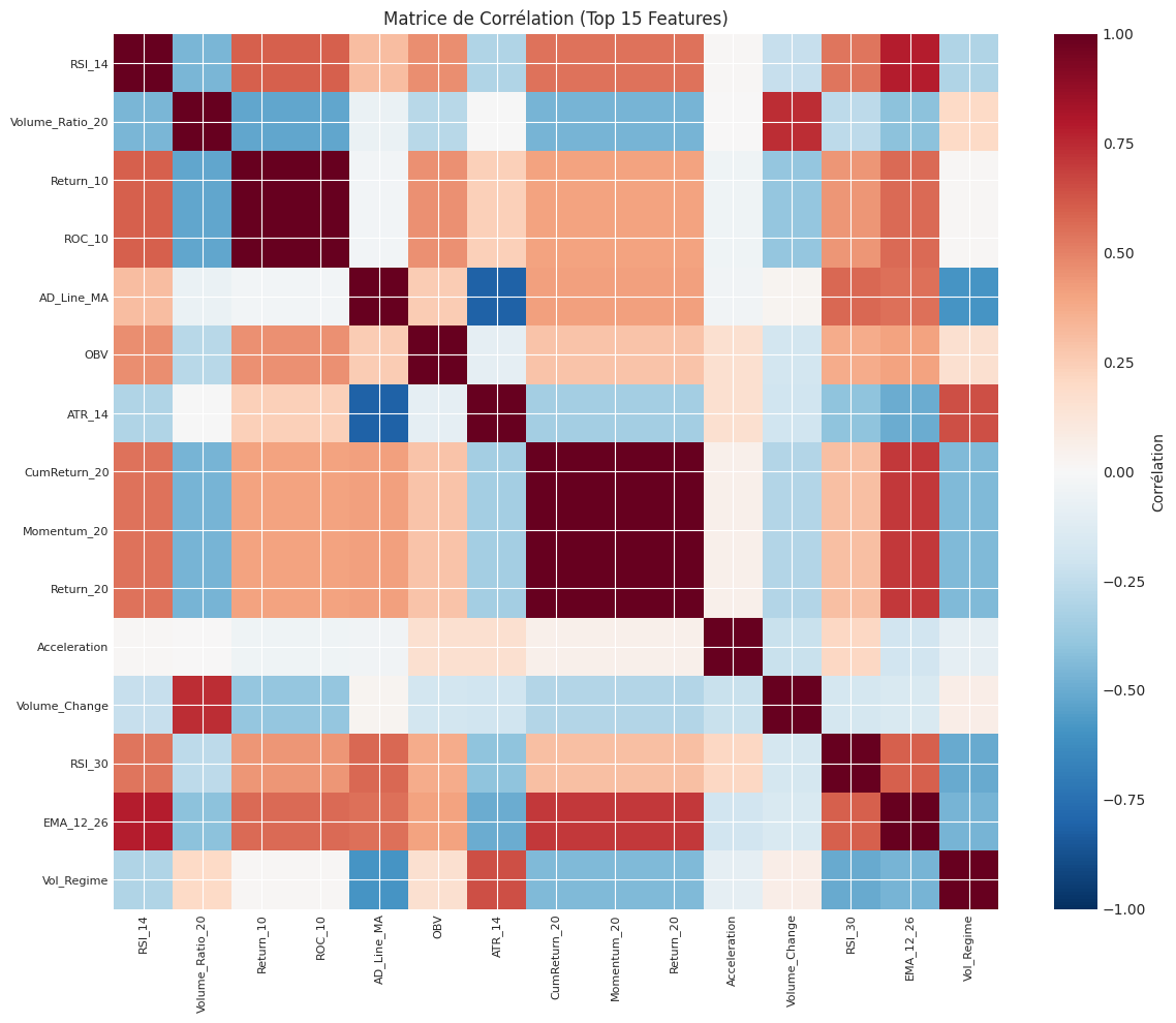
# Matrice de corrélation (top features) = mi_df.head(15 )['Feature' ].values= combined[top_features].corr()# Identifier les paires hautement corrélées = []for i in range (len (top_corr.columns)):for j in range (i+ 1 , len (top_corr.columns)):= top_corr.iloc[i, j]if abs (corr_val) > 0.9 :print ("Paires de features hautement corrélées (|r| > 0.9):" )if high_corr_pairs:for f1, f2, corr in high_corr_pairs:print (f" { f1} <-> { f2} : { corr:.3f} " )else :print (" Aucune - les features sont indépendantes" )# Visualiser la matrice de corrélation = plt.subplots(figsize= (12 , 10 ))= ax.imshow(top_corr, cmap= 'RdBu_r' , aspect= 'auto' , vmin=- 1 , vmax= 1 )range (len (top_corr.columns)))range (len (top_corr.columns)))= 90 , fontsize= 8 )= 8 )= ax, label= 'Corrélation' )'Matrice de Corrélation (Top 15 Features)' )'feature_correlation.png' , dpi= 150 )print ("Graphique sauvegardé." )
Paires de features hautement corrélées (|r| > 0.9):
  Return_10 <-> ROC_10: 1.000
  CumReturn_20 <-> Momentum_20: 1.000
  CumReturn_20 <-> Return_20: 1.000
  Momentum_20 <-> Return_20: 1.000
10. PCA - Réduction de Dimensionalité
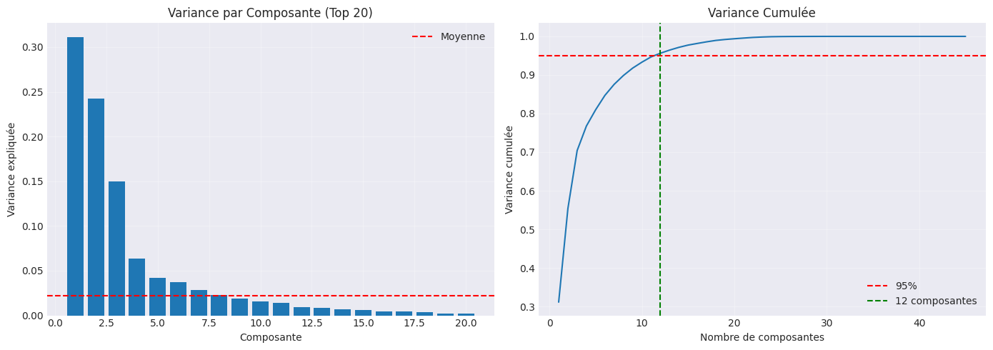
# Standardiser les features = StandardScaler()= scaler.fit_transform(X.fillna(0 ))# PCA = PCA()# Variance expliquée = pca.explained_variance_ratio_= np.cumsum(explained_var)# Nombre de composantes pour 95% de variance = np.argmax(cumsum_var >= 0.95 ) + 1 print ("=== Analyse PCA ===" )print (f"Nombre total de features: { len (X.columns)} " )print (f"Composantes pour 95% variance: { n_components_95} " )print (f"Réduction: { (1 - n_components_95/ len (X.columns))* 100 :.1f} %" )# Visualiser la variance expliquée = plt.subplots(1 , 2 , figsize= (14 , 5 ))# Variance par composante = axes[0 ]range (1 , 21 ), explained_var[:20 ])= 1 / len (X.columns), color= 'r' , linestyle= '--' , label= 'Moyenne' )'Composante' )'Variance expliquée' )'Variance par Composante (Top 20)' )True , alpha= 0.3 )# Variance cumulée = axes[1 ]range (1 , len (cumsum_var)+ 1 ), cumsum_var)= 0.95 , color= 'r' , linestyle= '--' , label= '95%' )= n_components_95, color= 'g' , linestyle= '--' , label= f' { n_components_95} composantes' )'Nombre de composantes' )'Variance cumulée' )'Variance Cumulée' )True , alpha= 0.3 )'pca_analysis.png' , dpi= 150 )print ("Graphique sauvegardé." )
=== Analyse PCA ===
Nombre total de features: 45
Composantes pour 95% variance: 12
Réduction: 73.3%
Interprétation: PCA
Variance expliquée : Combien d’information chaque composante captureComposantes principales : Combinaisons linéaires des features originalesRéduction : Moins de dimensions = modèle plus simple
Note : Pour l’interprétabilité, préférer les features originales. PCA pour la performance uniquement.
11. Pipeline de Feature Engineering Complet
def create_feature_pipeline(price_data, volume_data= None ):""" Pipeline complet de feature engineering. Args: price_data: DataFrame avec colonnes open, high, low, close volume_data: Série de volume (optionnel) Returns: DataFrame avec toutes les features """ = price_data['close' ]= price_data['high' ]= price_data['low' ]= pd.DataFrame(index= close.index)# 1. Features techniques 'RSI_14' ] = calculate_rsi(close, 14 )'RSI_30' ] = calculate_rsi(close, 30 )'EMA_20' ] = calculate_ema(close, 20 )'EMA_50' ] = calculate_ema(close, 50 )'EMA_200' ] = calculate_ema(close, 200 )'EMA_Ratio_50_200' ] = features['EMA_50' ] / features['EMA_200' ]# 2. Features momentum 'Return_1' ] = close.pct_change(1 )'Return_5' ] = close.pct_change(5 )'Return_20' ] = close.pct_change(20 )'Momentum_20' ] = (close - close.shift(20 )) / close.shift(20 )# 3. Features volatilité 'ATR_14' ] = calculate_atr(high, low, close, 14 )'Realized_Vol_20' ] = calculate_realized_vol(close, 20 )'Vol_Ratio' ] = (close.pct_change().rolling(5 ).std() / 20 ).std())# 4. Features volume (si disponible) if volume_data is not None :'Volume_Ratio' ] = volume_data / volume_data.rolling(20 ).mean()= calculate_obv(close, volume_data)'OBV_Signal' ] = (obv > obv.rolling(20 ).mean()).astype(int )# 5. Features temporelles — gerer MultiIndex (Symbol, datetime) if isinstance (close.index, pd.MultiIndex):= close.index.get_level_values(- 1 )else := close.index'Day_of_Week' ] = dt_index.dayofweek'Month' ] = dt_index.monthreturn features.fillna(0 )# Tester le pipeline = create_feature_pipeline(df, df['volume' ])print (f"Pipeline output: { len (pipeline_features.columns)} features" )print (f" \n Features créées:" )for i, col in enumerate (pipeline_features.columns, 1 ):print (f" { i} . { col} " )print (f" \n Derniers 3 jours:" )print (pipeline_features.iloc[- 3 :])
Pipeline output: 17 features

Features créées:
  1. RSI_14
  2. RSI_30
  3. EMA_20
  4. EMA_50
  5. EMA_200
  6. EMA_Ratio_50_200
  7. Return_1
  8. Return_5
  9. Return_20
  10. Momentum_20
  11. ATR_14
  12. Realized_Vol_20
  13. Vol_Ratio
  14. Volume_Ratio
  15. OBV_Signal
  16. Day_of_Week
  17. Month

Derniers 3 jours:
                     RSI_14  RSI_30  EMA_20  EMA_50     EMA_200  \
time
2025-12-29 16:00:00     0.0     0.0  396.33  396.33  396.329737
2025-12-30 16:00:00     0.0     0.0  396.33  396.33  396.329740
2025-12-31 16:00:00     0.0     0.0  396.33  396.33  396.329743

                     EMA_Ratio_50_200  Return_1  Return_5  Return_20  \
time
2025-12-29 16:00:00          1.000001       0.0       0.0        0.0
2025-12-30 16:00:00          1.000001       0.0       0.0        0.0
2025-12-31 16:00:00          1.000001       0.0       0.0        0.0

                     Momentum_20  ATR_14  Realized_Vol_20  Vol_Ratio  \
time
2025-12-29 16:00:00          0.0    2.67              0.0        0.0
2025-12-30 16:00:00          0.0    2.67              0.0        0.0
2025-12-31 16:00:00          0.0    2.67              0.0        0.0

                     Volume_Ratio  OBV_Signal  Day_of_Week  Month
time
2025-12-29 16:00:00           0.0           0            0     12
2025-12-30 16:00:00           0.0           0            1     12
2025-12-31 16:00:00           0.0           0            2     12
12. Meilleures Pratiques
1. Éviter le Data Leakage
Jamais utiliser les données du futur dans les featuresToujours utiliser .shift() pour les targets
Valider avec walk-forward, pas simple train/test split
2. Gérer les Valeurs Manquantes
Les indicateurs ont des warmup periods (ex: RSI = 14 jours)
Utiliser .fillna(0) ou .dropna() selon le cas
Documenter le warmup minimal pour chaque feature
3. Normalisation
StandardScaler pour les modèles linéaires (Ridge, SVM)Pas nécessaire pour Tree-based models (RF, XGBoost)
Toujours fit sur train set, transform sur test set
4. Feature Sélection
Utiliser Mutual Information pour la sélection
Éliminer les features avec MI < 0.001
Attention: la corrélation ≠ causalité
13. Checklist Feature Engineering
14. Ressources
QuantConnect Docs : https://www.quantconnect.com/docs/Feature Engineering : https://www.featurebook.org/ML for Trading : “Advances in Financial Machine Learning” by Marcos Lopez de Prado
Conclusion : Ce notebook fournit une base complète pour le feature engineering en trading. Utilisez ces features comme point de départ et adaptez-les à votre stratégie spécifique.