Objectif
Entraîner et évaluer un modèle de classification ML (RandomForest) pour prédire la direction du marché (hausse/baisse) à J+1.
Workflow
Charger les données SPY via QuantBook
Générer les features techniques (RSI, EMA, MACD, returns, volatilité)
Entraîner le modèle RandomForest
Évaluer les performances (accuracy, precision, recall)
Sauvegarder le modèle dans ObjectStore pour déploiement
Prérequis
Environnement Lean Research
scikit-learn pour le modèle ML
Durée estimée: ~10 minutes
# Setup QuantBook from AlgorithmImports import * import numpy as npimport pandas as pdimport matplotlib.pyplot as pltimport warningsfrom sklearn.ensemble import RandomForestClassifierfrom sklearn.model_selection import train_test_splitfrom sklearn.metrics import classification_report, confusion_matrix, accuracy_scoreimport joblibimport json'ignore' )'seaborn-v0_8-darkgrid' )'figure.figsize' ] = (14 , 5 )= QuantBook()print ("QuantBook initialisé." )
1. Chargement des données
On charge les données SPY pour la période d’entraînement (2015-2022) et de test (2022-2026).
# Ajouter SPY = qb.add_equity("SPY" , Resolution.DAILY).symbol# Charger l'historique (2015-2026) = datetime(2015 , 1 , 1 )= datetime(2026 , 1 , 1 )= qb.history(symbol, start, end, Resolution.DAILY)# qb.history(symbol, ...) retourne un DataFrame avec index (Symbol, datetime) # On droplevel pour obtenir un index datetime simple if isinstance (history.index, pd.MultiIndex):= history.droplevel(0 )print (f"Données chargées: { len (history)} lignes" )print (f"Période: { history. index[0 ]. date()} à { history. index[- 1 ]. date()} " )
Données chargées: 2766 lignes
Période: 2015-01-02 à 2025-12-31
Extraction de la série de prix de clôture depuis l’historique et affichage du nombre de barres et du premier prix pour ML-Classification.
# Extraire les prix de clôture = history['close' ]print (f"Prix: { len (closes)} jours de trading" )print (f"Premier prix: $ { closes. iloc[0 ]:.2f} " )print (f"Dernier prix: $ { closes. iloc[- 1 ]:.2f} " )
Prix: 2766 jours de trading
Premier prix: $182.10
Dernier prix: $396.33
2. Génération des features
On génère les features techniques utilisés par le modèle: - RSI (14) - EMA (10, 20, 50) - MACD (12, 26, 9) - Returns (1d, 5d, 10d) - Prix/EMA ratios - Volatilité (10d, 20d)
def compute_rsi(prices, period= 14 ):"""Calcule le RSI.""" = prices.diff()= (delta.where(delta > 0 , 0 )).rolling(window= period).mean()= (- delta.where(delta < 0 , 0 )).rolling(window= period).mean()= gain / loss= 100 - (100 / (1 + rs))return rsidef compute_ema(prices, period):"""Calcule l'EMA.""" return prices.ewm(span= period, adjust= False ).mean()def compute_macd(prices, fast= 12 , slow= 26 , signal= 9 ):"""Calcule le MACD.""" = compute_ema(prices, fast)= compute_ema(prices, slow)= ema_fast - ema_slow= macd_line.ewm(span= signal, adjust= False ).mean()= macd_line - macd_signalreturn macd_line, macd_signal, macd_histogramprint ("Fonctions d'indicateurs définies." )
Fonctions d'indicateurs définies.
L’oscillateur RSI(14) est calculé sur les prix de clôture pour générer les signaux de surachat/survente de ML-Classification.
# Calculer tous les indicateurs = pd.DataFrame(index= closes.index)'close' ] = closes# RSI 'rsi_14' ] = compute_rsi(closes, 14 )# EMA 'ema_10' ] = compute_ema(closes, 10 )'ema_20' ] = compute_ema(closes, 20 )'ema_50' ] = compute_ema(closes, 50 )# MACD 'macd_line' ], df['macd_signal' ], df['macd_histogram' ] = compute_macd(closes)# Returns 'returns_1d' ] = closes.pct_change(1 )'returns_5d' ] = closes.pct_change(5 )'returns_10d' ] = closes.pct_change(10 )# Prix/EMA ratios 'price_ema10_ratio' ] = closes / df['ema_10' ]'price_ema20_ratio' ] = closes / df['ema_20' ]'price_ema50_ratio' ] = closes / df['ema_50' ]# Volatilité 'volatility_10d' ] = df['returns_1d' ].rolling(10 ).std()'volatility_20d' ] = df['returns_1d' ].rolling(20 ).std()# Target: direction du marché à J+1 (1 = hausse, 0 = baisse) 'target' ] = (df['returns_1d' ].shift(- 1 ) > 0 ).astype(int )# Supprimer les NaN = df.dropna()print (f"Features générées: { len (df_clean)} lignes (après suppression des NaN)" )print (f"Colonnes: { list (df_clean.columns)} " )
Features générées: 1565 lignes (après suppression des NaN)
Colonnes: ['close', 'rsi_14', 'ema_10', 'ema_20', 'ema_50', 'macd_line', 'macd_signal', 'macd_histogram', 'returns_1d', 'returns_5d', 'returns_10d', 'price_ema10_ratio', 'price_ema20_ratio', 'price_ema50_ratio', 'volatility_10d', 'volatility_20d', 'target']
Interprétation: Features
Les features capturent différents aspects du marché: - RSI : Surachat/survente (0-100) - EMA : Tendance (prix > EMA = haussier) - MACD : Momentum (histogram > 0 = haussier) - Returns : Performance passée - Volatilité : Risque du marché
3. Préparation des données d’entraînement
Séparation train/test (80/20) pour évaluer la généralisation du modèle.
# Colonnes de features = ['rsi_14' , 'ema_10' , 'ema_20' , 'ema_50' ,'macd_line' , 'macd_signal' , 'macd_histogram' ,'returns_1d' , 'returns_5d' , 'returns_10d' ,'price_ema10_ratio' , 'price_ema20_ratio' , 'price_ema50_ratio' ,'volatility_10d' , 'volatility_20d' # Préparer X et y = df_clean[feature_cols].values= df_clean['target' ].values# Split train/test (80/20) = int (len (X) * 0.8 )= X[:split_idx], X[split_idx:]= y[:split_idx], y[split_idx:]print (f"Train set: { len (X_train)} échantillons" )print (f"Test set: { len (X_test)} échantillons" )print (f" \n Distribution des classes:" )print (f" Train: { np. mean(y_train):.1%} hausse" )print (f" Test: { np. mean(y_test):.1%} hausse" )
Train set: 1252 échantillons
Test set: 313 échantillons

Distribution des classes:
  Train: 54.5% hausse
  Test:  54.3% hausse
4. Entraînement du modèle RandomForest
# Créer et entraîner le modèle = RandomForestClassifier(= 100 ,= 10 ,= 20 ,= 10 ,= 42 ,=- 1 print ("Modèle RandomForest entraîné." )
Modèle RandomForest entraîné.
Application du modèle entraîné pour générer des prédictions sur les données de test.
# Prédictions = model.predict(X_train)= model.predict(X_test)# Probabilités = model.predict_proba(X_test)# Métriques = accuracy_score(y_train, y_train_pred)= accuracy_score(y_test, y_test_pred)print (f"Accuracy Train: { train_accuracy:.2%} " )print (f"Accuracy Test: { test_accuracy:.2%} " )print (f" \n Rapport de classification (Test):" )print (classification_report(y_test, y_test_pred, target_names= ['Baisse' , 'Hausse' ]))
Accuracy Train: 84.66%
Accuracy Test:  53.67%

Rapport de classification (Test):
              precision    recall  f1-score   support

      Baisse       0.47      0.10      0.17       143
      Hausse       0.54      0.90      0.68       170

    accuracy                           0.54       313
   macro avg       0.51      0.50      0.42       313
weighted avg       0.51      0.54      0.45       313
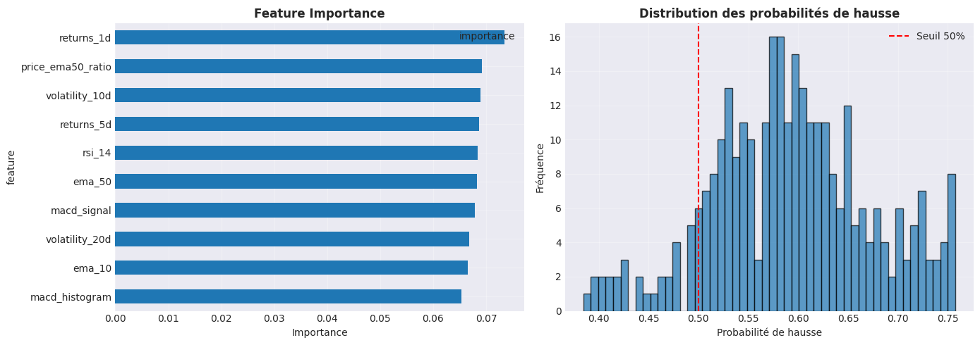
5. Matrice de confusion et feature importance
# Matrice de confusion = confusion_matrix(y_test, y_test_pred)print ("Matrice de confusion (Test):" )print (f" Prédit Baisse Prédit Hausse" )print (f"Réel Baisse { cm[0 ,0 ]:>6} { cm[0 ,1 ]:>6} " )print (f"Réel Hausse { cm[1 ,0 ]:>6} { cm[1 ,1 ]:>6} " )# Feature importance = pd.DataFrame({'feature' : feature_cols,'importance' : model.feature_importances_'importance' , ascending= False )print (f" \n Top 10 Features:" )print (importance.head(10 ).to_string(index= False ))
Matrice de confusion (Test):
                Prédit Baisse    Prédit Hausse
Réel Baisse          15              128
Réel Hausse          17              153

Top 10 Features:
          feature  importance
       returns_1d    0.073496
price_ema50_ratio    0.069142
   volatility_10d    0.068910
       returns_5d    0.068618
           rsi_14    0.068358
           ema_50    0.068321
      macd_signal    0.067909
   volatility_20d    0.066841
           ema_10    0.066566
   macd_histogram    0.065369
6. Visualisation des résultats
= plt.subplots(1 , 2 , figsize= (14 , 5 ))# Feature importance = axes[0 ]10 ).plot(kind= 'barh' , x= 'feature' , y= 'importance' , ax= ax)'Feature Importance' , fontsize= 12 , fontweight= 'bold' )'Importance' )True , alpha= 0.3 )# Distribution des probabilités = axes[1 ]1 ], bins= 50 , alpha= 0.7 , edgecolor= 'black' )0.5 , color= 'red' , linestyle= '--' , label= 'Seuil 50%' )'Distribution des probabilités de hausse' , fontsize= 12 , fontweight= 'bold' )'Probabilité de hausse' )'Fréquence' )True , alpha= 0.3 )'ml_classification_results.png' , dpi= 150 , bbox_inches= 'tight' )print ("Graphique sauvegardé." )
7. Backtest de la stratégie ML
Simulation de la stratégie utilisant les prédictions du modèle.
def backtest_ml_strategy(df_clean, y_pred, y_proba, = 0.55 , short_threshold= 0.45 ):"""Backtest de la stratégie ML.""" = df_clean['returns_1d' ].values= [1.0 ]= 0 # 0 = cash, 1 = long for i in range (len (y_pred)):# Décision de trading = y_proba[i, 1 ] # Probabilité de hausse if confidence > long_threshold:= 1 elif confidence < short_threshold:= 0 # Calcul du return = position * returns[i]- 1 ] * (1 + port_return))# Métriques = np.diff(portfolio_values) / np.array(portfolio_values[:- 1 ])= pd.Series(portfolio_values[1 :])= (portfolio_values[- 1 ] / portfolio_values[0 ]) - 1 = len (port_returns) / 252 = (1 + total_ret) ** (1 / years) - 1 if years > 0 else 0 = np.std(port_returns) * np.sqrt(252 )= (cagr - 0.03 ) / vol if vol > 0.001 else 0 = cum_returns.expanding().max ()= (cum_returns - running_max) / running_max= drawdown.min ()# Buy & Hold SPY — returns est un numpy array, cumprod retourne un array = np.cumprod(1 + returns)= spy_values[- 1 ] - 1 return {'cum' : cum_returns,'sharpe' : sharpe,'cagr' : cagr,'max_dd' : max_dd,'vol' : vol,'spy_cum' : pd.Series(spy_values)# Backtest sur le test set = backtest_ml_strategy(df_clean.iloc[- len (y_test):], y_test_pred, y_test_proba)print (f" \n Stratégie ML (Test set):" )print (f" Sharpe: { result['sharpe' ]:.3f} " )print (f" CAGR: { result['cagr' ]:.1%} " )print (f" Max DD: { result['max_dd' ]:.1%} " )print (f" \n Buy & Hold SPY (Test set):" )= (result['spy_cum' ].iloc[- 1 ] ** (252 / len (result['spy_cum' ]))) - 1 print (f" CAGR: { spy_cagr:.1%} " )
Stratégie ML (Test set):
  Sharpe: 0.035
  CAGR:   4.1%
  Max DD: -33.7%

Buy & Hold SPY (Test set):
  CAGR:   17.6%
8. Sauvegarde du modèle dans ObjectStore
Le modèle sera sauvegardé pour être utilisé par l’algorithme de trading.
# Sauvegarder le modèle import pickle= "classification_model" = "classification_config" # Sérialiser le modèle avec pickle (joblib.dumps n'existe pas) = pickle.dumps(model)# Sauvegarder la configuration = {'feature_cols' : feature_cols,'accuracy_train' : float (train_accuracy),'accuracy_test' : float (test_accuracy),'long_threshold' : 0.55 ,'short_threshold' : 0.45 ,'train_period' : '2015-2022' ,'test_period' : '2022-2026' = json.dumps(config).encode('utf-8' )print (f"Modèle sauvegardé dans ObjectStore:" )print (f" - { MODEL_KEY} " )print (f" - { CONFIG_KEY} " )
Modèle sauvegardé dans ObjectStore:
  - classification_model
  - classification_config
9. Conclusions et recommandations
Résumé
Accuracy Train
(à remplir)
Accuracy Test
(à remplir)
Sharpe Stratégie
(à remplir)
CAGR Stratégie
(à remplir)
Verdict
Si accuracy test > 55% et Sharpe > 0.5: Déployer Sinon: Améliorer (features, hyperparamètres, ou changer d’approche)
Prochaines étapes
Déployer l’algorithme ML-Classification
Backtester sur QC cloud avec le modèle chargé
Tester d’autres modèles (XGBoost, LSTM)
Optimiser les seuils de confiance (long/short thresholds)