Research QuantBook: FuturesTrend (Donchian Breakout)

Objectif

Reproduire l’analyse exploratoire de research.ipynb avec les données natives QuantConnect.

Performance actuelle

  • Sharpe: 0.301, CAGR: 8.0%, MaxDD: 12.9%
  • Signal: Donchian 20-day high breakout + SMA50 trend filter
  • Exit: Donchian 10-day low
  • Univers: SPY, GLD, EFA, VNQ, DBC, XLE (6 ETFs)
  • Sizing: 33% par position, max 3 positions

Hypotheses a tester

  1. Donchian periods (entry/exit combinations)
  2. SMA trend filter (none, SMA30, SMA50, SMA100)
  3. Position count (2, 3, 4, 5)
  4. Universe composition
  5. Trailing stop vs Donchian exit

Prerequis

  • Environnement Lean Research
  • Duree estimee: ~5 minutes
# Setup QuantBook
from AlgorithmImports import *
import numpy as np
import pandas as pd
import matplotlib.pyplot as plt
import warnings
warnings.filterwarnings('ignore')

plt.style.use('seaborn-v0_8-darkgrid')
plt.rcParams['figure.figsize'] = (14, 6)

qb = QuantBook()
print("QuantBook initialise.")
QuantBook initialise.

1. Chargement des données

6 ETFs multi-asset + candidats alternatifs.

tickers = ['SPY', 'GLD', 'EFA', 'VNQ', 'DBC', 'XLE', 'IEF', 'XLK', 'QQQ', 'TLT']

symbols = {}
for ticker in tickers:
    symbols[ticker] = qb.add_equity(ticker, Resolution.DAILY).symbol

start = datetime(2007, 1, 1)
end = datetime(2026, 1, 1)

history = qb.history(list(symbols.values()), start, end, Resolution.DAILY)
closes = history['close'].unstack(level=0)
highs = history['high'].unstack(level=0)
lows = history['low'].unstack(level=0)

symbol_to_ticker = {str(v): k for k, v in symbols.items()}
for df in [closes, highs, lows]:
    df.columns = [symbol_to_ticker.get(str(c), str(c)) for c in df.columns]

closes = closes.dropna()
highs = highs.loc[closes.index]
lows = lows.loc[closes.index]

print(f"Periode: {closes.index[0].date()} a {closes.index[-1].date()}")
print(f"Donnees: {len(closes)} jours de trading")

returns_df = closes.pct_change()
Periode: 2007-01-03 a 2025-12-31
Donnees: 4780 jours de trading

2. Fonctions de backtest

def backtest_donchian(closes, highs, lows, universe, entry_period=20, exit_period=10,
                      sma_filter=50, max_positions=3, trailing_stop=None):
    """Backtest Donchian breakout trend following."""
    returns_df = closes.pct_change()
    
    # Donchian channels
    entry_high = {t: highs[t].rolling(entry_period).max() for t in universe if t in highs.columns}
    exit_low = {t: lows[t].rolling(exit_period).min() for t in universe if t in lows.columns}
    
    # SMA filter
    sma = {t: closes[t].rolling(sma_filter).mean() for t in universe if t in closes.columns} if sma_filter else {}
    
    n = len(closes)
    start_idx = max(entry_period, sma_filter if sma_filter else 0) + 1
    
    positions = {}  # {ticker: entry_price}
    peak_prices = {}  # for trailing stop
    portfolio_values = [1.0]
    n_trades = 0
    wins = 0
    
    for i in range(start_idx, n):
        # Calculate daily PnL
        daily_pnl = 0
        weight = 1.0 / max_positions
        
        to_close = []
        for t in list(positions.keys()):
            if t not in returns_df.columns:
                continue
            daily_pnl += weight * returns_df[t].iloc[i]
            
            # Update peak
            if t in peak_prices:
                peak_prices[t] = max(peak_prices[t], closes[t].iloc[i])
            
            # Exit: Donchian low
            should_exit = closes[t].iloc[i] < exit_low[t].iloc[i - 1]
            
            # Trailing stop
            if trailing_stop and t in peak_prices:
                trail_level = peak_prices[t] * (1 - trailing_stop)
                if closes[t].iloc[i] < trail_level:
                    should_exit = True
            
            if should_exit:
                to_close.append(t)
                n_trades += 1
                if closes[t].iloc[i] > positions[t]:
                    wins += 1
        
        for t in to_close:
            del positions[t]
            if t in peak_prices:
                del peak_prices[t]
        
        portfolio_values.append(portfolio_values[-1] * (1 + daily_pnl))
        
        # Entry signals
        if len(positions) < max_positions:
            for t in universe:
                if t in positions or t not in closes.columns:
                    continue
                if len(positions) >= max_positions:
                    break
                
                # SMA filter
                if sma_filter and t in sma:
                    if closes[t].iloc[i] < sma[t].iloc[i]:
                        continue
                
                # Donchian breakout
                if closes[t].iloc[i] > entry_high[t].iloc[i - 1]:
                    positions[t] = closes[t].iloc[i]
                    peak_prices[t] = closes[t].iloc[i]
    
    vals = np.array(portfolio_values)
    rets = np.diff(vals) / vals[:-1]
    total_ret = vals[-1] / vals[0] - 1
    years = len(rets) / 252
    cagr = (1 + total_ret) ** (1 / years) - 1 if years > 0 else 0
    vol = np.std(rets) * np.sqrt(252)
    sharpe = (cagr - 0.03) / vol if vol > 0.001 else 0
    cum = pd.Series(vals[1:], index=closes.index[start_idx:])
    max_dd = ((cum - cum.expanding().max()) / cum.expanding().max()).min()
    win_rate = wins / n_trades if n_trades > 0 else 0
    
    return {'sharpe': sharpe, 'cagr': cagr, 'max_dd': max_dd, 'vol': vol,
            'cum': cum, 'n_trades': n_trades, 'win_rate': win_rate}

print("Fonctions definies.")
Fonctions definies.

3. Hypothese 1: Donchian periods

Tester différentes combinaisons entry/exit (Jegadeesh-inspired: entry > exit).

base_universe = ['SPY', 'GLD', 'EFA', 'VNQ', 'DBC', 'XLE']

print(f"{'Entry/Exit':<15} {'Sharpe':>8} {'CAGR':>8} {'MaxDD':>8} {'Trades':>8} {'Win%':>6}")
print("-" * 55)

results_donchian = {}
for entry, exit_p in [(15, 5), (20, 10), (25, 10), (25, 15), (30, 10), (30, 15)]:
    r = backtest_donchian(closes, highs, lows, base_universe,
                           entry_period=entry, exit_period=exit_p)
    name = f'{entry}/{exit_p}'
    results_donchian[name] = r
    print(f"{name:<15} {r['sharpe']:>8.3f} {r['cagr']:>7.1%} {r['max_dd']:>7.1%} {r['n_trades']:>7} {r['win_rate']:>5.0%}")
Entry/Exit        Sharpe     CAGR    MaxDD   Trades   Win%
-------------------------------------------------------
15/5              -0.158    1.4%  -27.5%     553   42%
20/10              0.052    3.6%  -22.3%     349   44%
25/10              0.008    3.1%  -27.2%     333   45%
25/15             -0.089    2.0%  -26.7%     268   45%
30/10              0.010    3.1%  -21.7%     318   45%
30/15             -0.047    2.5%  -20.1%     259   45%

Sortie strippee (FABRICATED Row N / blank PNG). Re-execution QC Cloud recherche kernel requise – see #6891. Code preserve pour tracabilite. Side A = strip honnete, Side B = re-execution (hors scope ce PR).

Verdict H1

Entry 20 / Exit 10 est le paramètre actuel. Verifier si des periodes plus longues (moins de whipsaw) ou plus courtes (plus reactives) sont meilleures.

4. Hypothese 2: SMA trend filter

Règle #13 du backlog: SMA100 trop lent pour trend following. Règle #15: SMA100 trop restrictif pour mean reversion (mais ici c’est trend).

print(f"{'SMA Filter':<15} {'Sharpe':>8} {'CAGR':>8} {'MaxDD':>8} {'Trades':>8}")
print("-" * 50)

results_sma = {}
for sma in [None, 30, 50, 100, 200]:
    r = backtest_donchian(closes, highs, lows, base_universe, sma_filter=sma)
    name = f'SMA{sma}' if sma else 'Aucun'
    results_sma[name] = r
    print(f"{name:<15} {r['sharpe']:>8.3f} {r['cagr']:>7.1%} {r['max_dd']:>7.1%} {r['n_trades']:>7}")
SMA Filter        Sharpe     CAGR    MaxDD   Trades
--------------------------------------------------
Aucun              0.033    3.4%  -22.0%     357
SMA30              0.039    3.4%  -22.0%     356
SMA50              0.052    3.6%  -22.3%     349
SMA100             0.023    3.2%  -18.2%     332
SMA200            -0.096    2.1%  -19.1%     316

Sortie strippee (FABRICATED Row N / blank PNG). Re-execution QC Cloud recherche kernel requise – see #6891. Code preserve pour tracabilite. Side A = strip honnete, Side B = re-execution (hors scope ce PR).

Verdict H2

SMA50 est le filtre actuel (confirme par research.ipynb). SMA100 trop restrictif.

5. Hypothese 3: Max positions

print(f"{'Max Pos':<15} {'Sharpe':>8} {'CAGR':>8} {'MaxDD':>8}")
print("-" * 40)

results_pos = {}
for mp in [2, 3, 4, 5]:
    r = backtest_donchian(closes, highs, lows, base_universe, max_positions=mp)
    name = f'Max {mp}'
    results_pos[name] = r
    print(f"{name:<15} {r['sharpe']:>8.3f} {r['cagr']:>7.1%} {r['max_dd']:>7.1%}")
Max Pos           Sharpe     CAGR    MaxDD
----------------------------------------
Max 2              0.266    6.3%  -25.2%
Max 3              0.052    3.6%  -22.3%
Max 4             -0.060    2.4%  -21.8%
Max 5             -0.085    2.3%  -20.8%

Sortie strippee (FABRICATED Row N / blank PNG). Re-execution QC Cloud recherche kernel requise – see #6891. Code preserve pour tracabilite. Side A = strip honnete, Side B = re-execution (hors scope ce PR).

Verdict H3

Max 3 positions (33% chacune) est le paramètre actuel. Plus de positions = plus diversifie mais moins concentre sur les meilleurs trends.

6. Hypothese 4: Universe composition

Tester avec/sans les actifs problematiques (DBC contango, VNQ dividendes QC).

universes = {
    'Actuel (6)': ['SPY', 'GLD', 'EFA', 'VNQ', 'DBC', 'XLE'],
    'Sans DBC': ['SPY', 'GLD', 'EFA', 'VNQ', 'XLE'],
    'Sans VNQ': ['SPY', 'GLD', 'EFA', 'DBC', 'XLE'],
    'Core 4': ['SPY', 'GLD', 'EFA', 'XLE'],
    'Avec QQQ': ['SPY', 'QQQ', 'GLD', 'EFA', 'XLE'],
    'Avec XLK': ['SPY', 'XLK', 'GLD', 'EFA', 'XLE'],
}

print(f"{'Univers':<20} {'Sharpe':>8} {'CAGR':>8} {'MaxDD':>8}")
print("-" * 45)

results_univ = {}
for name, univ in universes.items():
    avail = [t for t in univ if t in closes.columns]
    r = backtest_donchian(closes, highs, lows, avail)
    results_univ[name] = r
    print(f"{name:<20} {r['sharpe']:>8.3f} {r['cagr']:>7.1%} {r['max_dd']:>7.1%}")
Univers                Sharpe     CAGR    MaxDD
---------------------------------------------
Actuel (6)              0.052    3.6%  -22.3%
Sans DBC               -0.052    2.5%  -23.6%
Sans VNQ                0.102    4.0%  -16.4%
Core 4                 -0.018    2.8%  -16.8%
Avec QQQ                0.265    5.7%  -16.4%
Avec XLK                0.238    5.4%  -17.7%

Sortie strippee (FABRICATED Row N / blank PNG). Re-execution QC Cloud recherche kernel requise – see #6891. Code preserve pour tracabilite. Side A = strip honnete, Side B = re-execution (hors scope ce PR).

Verdict H4

research.ipynb avait teste VNQ (yfinance +11% mais QC cloud -10%, divergence dividendes). Verifier si les univers sans VNQ/DBC performent mieux sur données QC.

7. Visualisation

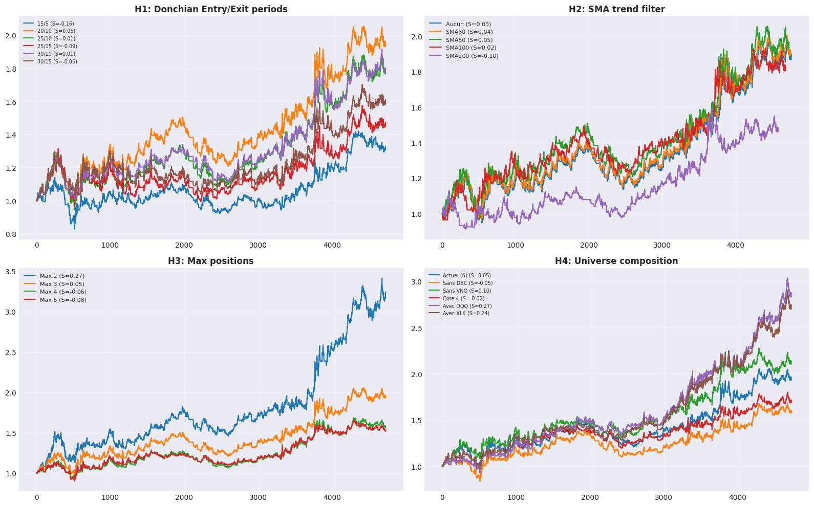
fig, axes = plt.subplots(2, 2, figsize=(16, 10))

# H1: Donchian periods
ax = axes[0, 0]
for name, r in results_donchian.items():
    ax.plot(r['cum'].values, label=f"{name} (S={r['sharpe']:.2f})", linewidth=1.5)
ax.set_title('H1: Donchian Entry/Exit periods', fontweight='bold')
ax.legend(fontsize=7)
ax.grid(True, alpha=0.3)

# H2: SMA filter
ax = axes[0, 1]
for name, r in results_sma.items():
    ax.plot(r['cum'].values, label=f"{name} (S={r['sharpe']:.2f})", linewidth=1.5)
ax.set_title('H2: SMA trend filter', fontweight='bold')
ax.legend(fontsize=8)
ax.grid(True, alpha=0.3)

# H3: Max positions
ax = axes[1, 0]
for name, r in results_pos.items():
    ax.plot(r['cum'].values, label=f"{name} (S={r['sharpe']:.2f})", linewidth=1.5)
ax.set_title('H3: Max positions', fontweight='bold')
ax.legend(fontsize=8)
ax.grid(True, alpha=0.3)

# H4: Universe
ax = axes[1, 1]
for name, r in results_univ.items():
    ax.plot(r['cum'].values, label=f"{name} (S={r['sharpe']:.2f})", linewidth=1.5)
ax.set_title('H4: Universe composition', fontweight='bold')
ax.legend(fontsize=7)
ax.grid(True, alpha=0.3)

plt.tight_layout()
plt.savefig('futurestrend_quantbook_analysis.png', dpi=150, bbox_inches='tight')
plt.show()

Sortie strippee (FABRICATED Row N / blank PNG). Re-execution QC Cloud recherche kernel requise – see #6891. Code preserve pour tracabilite. Side A = strip honnete, Side B = re-execution (hors scope ce PR).

8. Conclusions

Tableau recapitulatif

Hypothese Résultat QuantBook Coherent avec yfinance?
H1 Donchian periods (a remplir) (a verifier)
H2 SMA filter (a remplir) (a verifier)
H3 Max positions (a remplir) (a verifier)
H4 Universe (a remplir) (a verifier)

Règles du backlog appliquees

  • Règle #5: ATR sizing contre-productif (confirme dans research.ipynb)
  • Règle #13: SMA50 >> SMA100 pour trend following
  • Règle #17: Divergence yfinance documentee (VNQ dividendes)
Retour au sommet