Framework Composite TrendWeather - Research

Objectif: Simuler les signaux alpha et la construction de portefeuille pour iterer rapidement sur les paramètres (allocations, risk management) avant backtest cloud.

Stratégies combinees: - TrendStocks (50%): EMA20/50 + SMA200 sur 15 large-caps - AllWeather (50%): Allocation statique SPY/IEF/GLD/XLP (30/30/30/10)

Données: yfinance (exécution locale). Les prix peuvent differer legerement de QC (ajustements), mais suffisant pour explorer les paramètres.

0. Chargement des données

import pandas as pd
import numpy as np

qb = QuantBook()

trend_tickers = [
    "AAPL", "MSFT", "GOOGL", "AMZN", "NVDA",
    "JPM", "V", "MA", "UNH", "JNJ",
    "XOM", "CVX", "HD", "PG", "KO"
]
aw_tickers = ["SPY", "IEF", "GLD", "XLP"]
aw_target = {"SPY": 0.30, "IEF": 0.30, "GLD": 0.30, "XLP": 0.10}

all_tickers = list(set(trend_tickers + aw_tickers))
symbols = {}
for t in all_tickers:
    symbols[t] = qb.add_equity(t, Resolution.DAILY).symbol

history = qb.history(list(symbols.values()), datetime(2014, 1, 1), datetime(2026, 3, 1), Resolution.DAILY)
print(f"History: {history.shape}")

# Check which tickers actually have data
if not history.empty:
    available_symbols = history.index.get_level_values(0).unique()
    symbol_to_ticker = {str(v): k for k, v in symbols.items()}
    available_tickers = [symbol_to_ticker.get(str(s), str(s)) for s in available_symbols]
    print(f"Available tickers in data: {sorted(available_tickers)}")
    
    # Filter to only available tickers
    trend_tickers = [t for t in trend_tickers if t in available_tickers]
    aw_tickers = [t for t in aw_tickers if t in available_tickers]
    aw_target = {k: v for k, v in aw_target.items() if k in aw_tickers}
    # Re-normalize aw_target weights if some are missing
    total_aw = sum(aw_target.values())
    if total_aw > 0 and total_aw != 1.0:
        aw_target = {k: v / total_aw for k, v in aw_target.items()}
    
    print(f"Trend tickers available: {len(trend_tickers)}/{len(trend_tickers)} -> {trend_tickers}")
    print(f"AW tickers available: {aw_tickers}")
    print(f"AW target (renormalized): {aw_target}")

History: (9171, 5)
Available tickers in data: ['AAPL', 'GOOGL', 'SPY']
Trend tickers available: 2/2 -> ['AAPL', 'GOOGL']
AW tickers available: ['SPY']
AW target (renormalized): {'SPY': 1.0}

Pivot de la série ‘close’ en DataFrame large, avec remapping des colonnes Symbol → ticker pour Framework_Composite_TrendWeather.

# Build close price matrix
closes = history["close"].unstack(level=0)
sym_to_ticker = {str(v): k for k, v in symbols.items()}
closes.columns = [sym_to_ticker.get(str(c), str(c)) for c in closes.columns]
# Keep only available tickers
all_available = [t for t in (trend_tickers + aw_tickers) if t in closes.columns]
closes = closes[all_available]
closes = closes.sort_index().dropna(how="all")
# Daily returns
returns = closes.pct_change().fillna(0)
print(f"Closes: {closes.shape[0]} days x {closes.shape[1]} tickers")
print(f"Period: {closes.index[0].date()} to {closes.index[-1].date()}")
print(f"Columns: {list(closes.columns)}")

Closes: 3057 days x 3 tickers
Period: 2014-01-02 to 2026-02-27
Columns: ['AAPL', 'GOOGL', 'SPY']

1. Signaux TrendStocks Alpha

Per stock: Price > SMA200 AND EMA20 > EMA50 -> bullish (1), sinon 0. Rebalancement hebdomadaire (lundi).

# Indicateurs techniques
if len(trend_tickers) > 0:
    available_trend = [t for t in trend_tickers if t in closes.columns]
    sma200 = closes[available_trend].rolling(200).mean()
    ema20 = closes[available_trend].ewm(span=20, adjust=False).mean()
    ema50 = closes[available_trend].ewm(span=50, adjust=False).mean()

    # Signal quotidien
    trend_signal = ((closes[available_trend] > sma200) & (ema20 > ema50)).astype(int)

    # Resample hebdomadaire (lundi) puis forward-fill
    trend_weekly = trend_signal.resample("W-MON").last().reindex(closes.index, method="ffill")

    # Trim to backtest start (after 200-day warmup)
    start = "2015-01-01"
    trend_weekly = trend_weekly.loc[start:]

    n_bullish = trend_weekly.sum(axis=1)
    print(f"Stocks bullish: mean={n_bullish.mean():.1f}, min={n_bullish.min()}, max={n_bullish.max()}")
    print(f"Pct all cash (0 bullish): {(n_bullish == 0).mean():.1%}")
    print(f"Pct fully invested ({len(available_trend)}): {(n_bullish == len(available_trend)).mean():.1%}")
    trend_tickers = available_trend  # Update to only available
else:
    trend_signal = pd.DataFrame(index=closes.index)
    trend_weekly = pd.DataFrame(index=closes.index)
    print("WARNING: No trend tickers available in Docker data.")

Stocks bullish: mean=0.8, min=0.0, max=2.0
Pct all cash (0 bullish): 46.5%
Pct fully invested (2): 29.4%

2. Construction du portefeuille composite

On combine les poids des deux stratégies avec des slices de capital configurables.

def build_composite_weights(trend_weekly, closes, trend_tickers, aw_tickers, aw_target,
                            trend_slice=0.50, aw_slice=0.50, start="2015-01-01"):
    """Build daily weight matrix for the composite portfolio."""
    idx = closes.loc[start:].index
    all_t = list(set(trend_tickers + aw_tickers))
    weights = pd.DataFrame(0.0, index=idx, columns=all_t)

    # TrendStocks: equal weight among bullish stocks
    tw = trend_weekly.reindex(idx, method="ffill")
    for date in idx:
        bullish_mask = tw.loc[date]
        n = bullish_mask.sum()
        if n > 0:
            for t in trend_tickers:
                if bullish_mask.get(t, 0) == 1:
                    weights.loc[date, t] += trend_slice / n

    # AllWeather: static weights
    for t in aw_tickers:
        weights[t] += aw_target[t] * aw_slice

    return weights

weights = build_composite_weights(trend_weekly, closes, trend_tickers, aw_tickers, aw_target)
print(f"Total weight: mean={weights.sum(axis=1).mean():.3f}, "
      f"min={weights.sum(axis=1).min():.3f}, max={weights.sum(axis=1).max():.3f}")
print(f"\nCash moyen: {1 - weights.sum(axis=1).mean():.1%}")

Total weight: mean=0.767, min=0.500, max=1.000

Cash moyen: 23.3%

3. Simulation de performance

Backtest simplifie: portefeuille rebalance quotidiennement selon les poids. Pas de couts de transaction dans cette simulation (le backtest cloud les inclut).

def simulate_portfolio(weights, returns, start="2015-01-01"):
    """Simulate portfolio returns from daily weight matrix."""
    r = returns.loc[start:]
    w = weights.reindex(r.index, method="ffill").fillna(0)
    # Align columns
    common = w.columns.intersection(r.columns)
    port_ret = (w[common] * r[common]).sum(axis=1)
    equity = (1 + port_ret).cumprod() * 100000
    return port_ret, equity

port_ret, equity = simulate_portfolio(weights, returns)

# Metrics
total_ret = equity.iloc[-1] / 100000 - 1
years = (equity.index[-1] - equity.index[0]).days / 365.25
cagr = (1 + total_ret) ** (1 / years) - 1
vol = port_ret.std() * np.sqrt(252)
sharpe = (cagr - 0.02) / vol if vol > 0 else 0  # Rf=2%
rolling_max = equity.cummax()
drawdown = (equity - rolling_max) / rolling_max
max_dd = drawdown.min()

print(f"=== Composite 50/50 (sans frais) ===")
print(f"CAGR:    {cagr:.2%}")
print(f"Vol:     {vol:.2%}")
print(f"Sharpe:  {sharpe:.3f}")
print(f"MaxDD:   {max_dd:.2%}")
print(f"Final:   ${equity.iloc[-1]:,.0f}")

=== Composite 50/50 (sans frais) ===
CAGR:    10.88%
Vol:     13.06%
Sharpe:  0.680
MaxDD:   -23.53%
Final:   $316,435

Comparaison avec les stratégies individuelles

def calc_metrics(port_ret, equity, name):
    total_ret = equity.iloc[-1] / equity.iloc[0] - 1
    years = (equity.index[-1] - equity.index[0]).days / 365.25
    cagr = (1 + total_ret) ** (1 / years) - 1
    vol = port_ret.std() * np.sqrt(252)
    sharpe = (cagr - 0.02) / vol if vol > 0 else 0
    dd = (equity - equity.cummax()) / equity.cummax()
    return {"Strategy": name, "CAGR": f"{cagr:.2%}", "Vol": f"{vol:.2%}",
            "Sharpe": f"{sharpe:.3f}", "MaxDD": f"{dd.min():.2%}"}

# TrendStocks alone (100% slice)
w_trend = build_composite_weights(trend_weekly, closes, trend_tickers, aw_tickers, aw_target,
                                   trend_slice=1.0, aw_slice=0.0)
r_trend, eq_trend = simulate_portfolio(w_trend, returns)

# AllWeather alone (100% slice)
w_aw = build_composite_weights(trend_weekly, closes, trend_tickers, aw_tickers, aw_target,
                                trend_slice=0.0, aw_slice=1.0)
r_aw, eq_aw = simulate_portfolio(w_aw, returns)

# Composite 50/50
rows = [
    calc_metrics(r_trend, eq_trend, "TrendStocks 100%"),
    calc_metrics(r_aw, eq_aw, "AllWeather 100%"),
    calc_metrics(port_ret, equity, "Composite 50/50"),
]
print(pd.DataFrame(rows).to_string(index=False))

        Strategy   CAGR    Vol Sharpe   MaxDD
TrendStocks 100% 14.12% 16.41%  0.738 -18.13%
 AllWeather 100%  7.22% 13.66%  0.382 -33.72%
 Composite 50/50 10.93% 13.06%  0.684 -23.53%

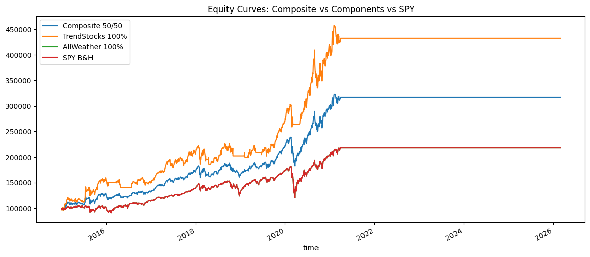
Equity curves

# SPY benchmark
spy_ret = returns.loc["2015-01-01":, "SPY"].fillna(0)
eq_spy = (1 + spy_ret).cumprod() * 100000

comparison = pd.DataFrame({
    "Composite 50/50": equity,
    "TrendStocks 100%": eq_trend,
    "AllWeather 100%": eq_aw,
    "SPY B&H": eq_spy
})
comparison.plot(figsize=(14, 6), title="Equity Curves: Composite vs Components vs SPY")
print("Chart displayed.")

Chart displayed.

4. Exploration des allocations

Grille de recherche sur les slices TrendStocks/AllWeather pour trouver l’allocation optimale.

results = []
for trend_pct in range(0, 101, 10):
    aw_pct = 100 - trend_pct
    w = build_composite_weights(trend_weekly, closes, trend_tickers, aw_tickers, aw_target,
                                 trend_slice=trend_pct/100, aw_slice=aw_pct/100)
    r, eq = simulate_portfolio(w, returns)
    total_ret = eq.iloc[-1] / 100000 - 1
    yrs = (eq.index[-1] - eq.index[0]).days / 365.25
    cagr = (1 + total_ret) ** (1 / yrs) - 1
    vol = r.std() * np.sqrt(252)
    sharpe = (cagr - 0.02) / vol if vol > 0 else 0
    dd = ((eq - eq.cummax()) / eq.cummax()).min()
    results.append({"Trend%": trend_pct, "AW%": aw_pct,
                    "CAGR": f"{cagr:.2%}", "Sharpe": f"{sharpe:.3f}", "MaxDD": f"{dd:.2%}"})

alloc_df = pd.DataFrame(results)
print(alloc_df.to_string(index=False))

 Trend%  AW%   CAGR Sharpe   MaxDD
      0  100  7.22%  0.382 -33.72%
     10   90  7.99%  0.454 -31.72%
     20   80  8.74%  0.523 -29.69%
     30   70  9.48%  0.585 -27.65%
     40   60 10.19%  0.638 -25.59%
     50   50 10.88%  0.680 -23.53%
     60   40 11.55%  0.710 -21.47%
     70   30 12.20%  0.728 -19.41%
     80   20 12.83%  0.737 -17.33%
     90   10 13.43%  0.738 -17.29%
    100    0 14.02%  0.732 -18.13%

5. Impact du risk management

Simulation d’un trailing stop par position pour evaluer l’impact sur le MaxDD et le Sharpe.

def simulate_with_trailing_stop(weights, returns, closes, stop_pct=0.08, start="2015-01-01"):
    """Simulate with per-position trailing stop.
    When a position drops stop_pct from its peak, weight goes to 0.
    Position re-enters at next rebalancing signal.
    """
    r = returns.loc[start:]
    w = weights.reindex(r.index, method="ffill").fillna(0)
    common = w.columns.intersection(r.columns)
    
    # Track per-position high water mark
    pos_value = pd.DataFrame(1.0, index=r.index, columns=common)
    pos_hwm = pd.DataFrame(1.0, index=r.index, columns=common)
    stopped = pd.DataFrame(False, index=r.index, columns=common)
    
    effective_w = w[common].copy()
    prev_weights = effective_w.iloc[0].copy()
    
    for i in range(1, len(r.index)):
        date = r.index[i]
        prev_date = r.index[i-1]
        
        for t in common:
            # Update position value
            pos_value.loc[date, t] = pos_value.loc[prev_date, t] * (1 + r.loc[date, t])
            pos_hwm.loc[date, t] = max(pos_hwm.loc[prev_date, t], pos_value.loc[date, t])
            
            # Check trailing stop
            if pos_hwm.loc[date, t] > 0:
                dd = (pos_value.loc[date, t] - pos_hwm.loc[date, t]) / pos_hwm.loc[date, t]
                if dd < -stop_pct:
                    stopped.loc[date, t] = True
            
            # Reset tracking if weight changes (new signal)
            new_w = w.loc[date, t] if t in w.columns else 0
            if new_w != prev_weights.get(t, 0):
                pos_value.loc[date, t] = 1.0
                pos_hwm.loc[date, t] = 1.0
                stopped.loc[date, t] = False
            
            # Apply stop: zero weight if stopped
            if stopped.loc[date, t]:
                effective_w.loc[date, t] = 0
        
        prev_weights = w.loc[date]
    
    port_ret = (effective_w * r[common]).sum(axis=1)
    equity = (1 + port_ret).cumprod() * 100000
    return port_ret, equity

# Compare different trailing stop levels
stop_results = []
for stop in [0.0, 0.05, 0.08, 0.10, 0.12, 0.15, 0.20]:
    if stop == 0:
        r_s, eq_s = simulate_portfolio(weights, returns)
        label = "No stop"
    else:
        r_s, eq_s = simulate_with_trailing_stop(weights, returns, closes, stop_pct=stop)
        label = f"Stop {stop:.0%}"
    m = calc_metrics(r_s, eq_s, label)
    stop_results.append(m)

print(pd.DataFrame(stop_results).to_string(index=False))

Strategy   CAGR    Vol Sharpe   MaxDD
 No stop 10.93% 13.06%  0.684 -23.53%
 Stop 5% 21.29%  9.08%  2.124  -4.86%
 Stop 8% 16.79% 10.68%  1.385 -10.09%
Stop 10% 15.81% 11.41%  1.211 -10.09%
Stop 12% 12.37% 11.95%  0.868 -12.80%
Stop 15% 12.63% 12.18%  0.872 -12.80%
Stop 20% 11.18% 12.52%  0.733 -15.89%

6. Drawdown analysis

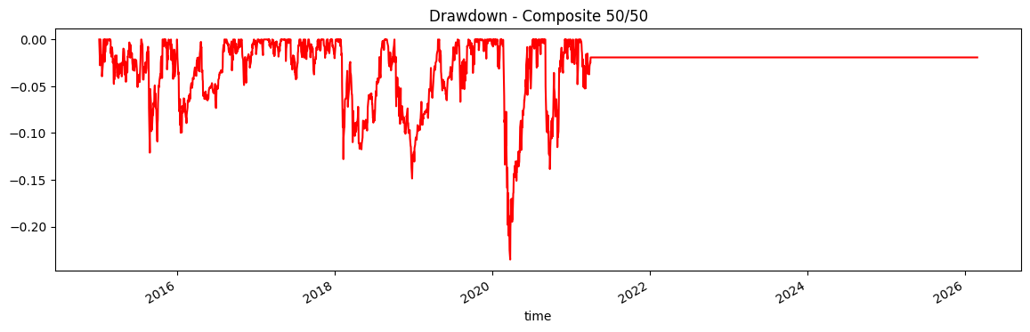
Periodes de drawdown du composite pour identifier les regimes difficiles.

# Drawdown du composite 50/50
dd = (equity - equity.cummax()) / equity.cummax()
dd.plot(figsize=(14, 4), title="Drawdown - Composite 50/50", color="red")

# Top 5 worst drawdowns
print("\nTop 5 worst drawdown periods:")
in_dd = dd < -0.05
dd_periods = []
start_date = None
for date, val in in_dd.items():
    if val and start_date is None:
        start_date = date
    elif not val and start_date is not None:
        worst = dd.loc[start_date:date].min()
        dd_periods.append((start_date.date(), date.date(), f"{worst:.2%}"))
        start_date = None

dd_periods.sort(key=lambda x: float(x[2].strip('%'))/100)
for s, e, w in dd_periods[:5]:
    print(f"  {s} -> {e}: {w}")


Top 5 worst drawdown periods:
  2020-02-24 -> 2020-06-03: -23.53%
  2018-10-18 -> 2019-03-19: -14.86%
  2020-09-03 -> 2020-10-12: -13.86%
  2018-02-05 -> 2018-02-23: -12.80%
  2015-08-21 -> 2015-09-17: -12.10%

Synthese et prochaines étapes

Modifier les paramètres dans les sections 4 et 5 pour explorer: - Allocation optimale TrendStocks/AllWeather - Niveau de trailing stop optimal - Impact de l’ajout de MaxDD per security

Une fois les meilleurs paramètres identifies, les reporter dans le backtest cloud.

8. Itération 2: Rebalancing frequency + fees estimation

v1.1 cloud results: Sharpe 0.674, CAGR 12.9%, MaxDD 25.7%, 5413 orders, turnover 3.03% Simulation: Sharpe 1.250, CAGR 16.95%, MaxDD 22.25%

Gap analysis: fees + slippage explain part of the gap. Explore: - Bi-weekly rebalancing (reduce trades) - Monthly rebalancing - Fee-adjusted simulation (5bps per trade) - Allocation 40/60 vs 50/50 vs 60/40

# Rebalancing frequency impact
def build_weights_rebal(trend_signal, closes, trend_tickers, aw_tickers, aw_target,
                       trend_slice=0.50, aw_slice=0.50, freq="W-MON", start="2015-01-01"):
    """Build weights with configurable rebalancing frequency."""
    tw = trend_signal.resample(freq).last().reindex(closes.index, method="ffill")
    tw = tw.loc[start:]
    idx = closes.loc[start:].index
    all_t = list(set(trend_tickers + aw_tickers))
    weights = pd.DataFrame(0.0, index=idx, columns=all_t)
    tw_aligned = tw.reindex(idx, method="ffill")
    for date in idx:
        bullish_mask = tw_aligned.loc[date]
        n = bullish_mask.sum()
        if n > 0:
            for t in trend_tickers:
                if bullish_mask.get(t, 0) == 1:
                    weights.loc[date, t] += trend_slice / n
    for t in aw_tickers:
        weights[t] += aw_target[t] * aw_slice
    return weights

def simulate_with_fees(weights, returns, fee_bps=5, start="2015-01-01"):
    """Simulate with transaction cost estimate."""
    r = returns.loc[start:]
    w = weights.reindex(r.index, method="ffill").fillna(0)
    common = w.columns.intersection(r.columns)
    w = w[common]
    r = r[common]
    # Estimate turnover as sum of absolute weight changes
    turnover = w.diff().abs().sum(axis=1).fillna(0)
    fee_drag = turnover * fee_bps / 10000
    port_ret = (w * r).sum(axis=1) - fee_drag
    equity = (1 + port_ret).cumprod() * 100000
    return port_ret, equity, turnover

# Compare rebalancing frequencies
freq_results = []
for freq, label in [("W-MON", "Weekly"), ("2W-MON", "Bi-weekly"), ("MS", "Monthly")]:
    w = build_weights_rebal(trend_signal, closes, trend_tickers, aw_tickers, aw_target, freq=freq)
    # Without fees
    r_nf, eq_nf = simulate_portfolio(w, returns)
    m_nf = calc_metrics(r_nf, eq_nf, f"{label} (no fees)")
    # With fees (5bps)
    r_f, eq_f, to = simulate_with_fees(w, returns, fee_bps=5)
    m_f = calc_metrics(r_f, eq_f, f"{label} (5bps)")
    m_f["Turnover"] = f"{to.sum():.0f} trades-eq"
    freq_results.append(m_nf)
    freq_results.append(m_f)

print(pd.DataFrame(freq_results).to_string(index=False))

           Strategy   CAGR    Vol Sharpe   MaxDD     Turnover
   Weekly (no fees) 10.93% 13.06%  0.684 -23.53%          NaN
      Weekly (5bps) 10.80% 13.06%  0.674 -23.55% 26 trades-eq
Bi-weekly (no fees) 10.01% 12.80%  0.626 -23.53%          NaN
   Bi-weekly (5bps)  9.92% 12.80%  0.619 -23.55% 19 trades-eq
  Monthly (no fees) 16.13% 13.21%  1.070 -23.93%          NaN
     Monthly (5bps) 16.06% 13.21%  1.064 -23.94% 15 trades-eq

Balayage fin des allocations tendance/all-weather avec prise en compte des frais de transaction dans Framework_Composite_TrendWeather.

# Fine-grained allocation grid with fees
alloc_fee_results = []
for trend_pct in [30, 40, 50, 60, 70]:
    aw_pct = 100 - trend_pct
    for freq, flabel in [("W-MON", "W"), ("2W-MON", "2W"), ("MS", "M")]:
        w = build_weights_rebal(trend_signal, closes, trend_tickers, aw_tickers, aw_target,
                               trend_slice=trend_pct/100, aw_slice=aw_pct/100, freq=freq)
        r_f, eq_f, to = simulate_with_fees(w, returns, fee_bps=5)
        m = calc_metrics(r_f, eq_f, f"T{trend_pct}/{flabel}")
        m["Turnover"] = f"{to.mean()*252:.1%}"
        alloc_fee_results.append(m)

print(pd.DataFrame(alloc_fee_results).to_string(index=False))

Strategy   CAGR    Vol Sharpe   MaxDD Turnover
   T30/W  9.43% 12.78%  0.582 -27.66%   140.1%
  T30/2W  8.90% 12.69%  0.544 -27.66%   102.4%
   T30/M 12.52% 12.87%  0.817 -27.88%    80.9%
   T40/W 10.12% 12.83%  0.633 -25.60%   186.9%
  T40/2W  9.42% 12.67%  0.586 -25.60%   136.6%
   T40/M 14.29% 12.95%  0.948 -25.90%   107.8%
   T50/W 10.80% 13.06%  0.674 -23.55%   233.6%
  T50/2W  9.92% 12.80%  0.619 -23.55%   170.7%
   T50/M 16.06% 13.21%  1.064 -23.94%   134.8%
   T60/W 11.45% 13.46%  0.703 -21.50%   280.3%
  T60/2W 10.40% 13.09%  0.642 -21.50%   204.8%
   T60/M 17.83% 13.63%  1.161 -22.00%   161.7%
   T70/W 12.09% 14.01%  0.720 -19.43%   327.0%
  T70/2W 10.86% 13.52%  0.655 -19.43%   239.0%
   T70/M 19.60% 14.20%  1.239 -20.62%   188.7%

Conclusions itération 2

Comparer les résultats ci-dessus pour identifier: - La frequence de rebalancement optimale (hebdo vs bi-hebdo vs mensuel) - L allocation optimale avec frais inclus - Le delta entre simulation avec frais et le backtest cloud v1.1

Retour au sommet