Objectif
Analyser la stratégie EMA crossover sur SPY (S&P 500 ETF).
Stratégie
Underlying : SPY (S&P 500 ETF)Signal : EMA(20) > EMA(60) pour long, flat sinonCooldown : 3 jours après exit (évite whipsaws)Position : 95% investi quand signal long
Hypothèses à tester
Période EMA: (10/40), (20/50), (20/60)
Cooldown: 0, 3, 5 jours
Trailing stop: aucun vs 5%
Prérequis
Environnement Lean Research
Données SPY
Durée estimée: ~6 minutes
Note de recherche (v2.0) : - EMA 20/60 sélectionné via robustesse IS/OOS = 1.55 - Cooldown 3d élimine 1 whipsaw sur 11 ans (+4.6% Sharpe) - Trailing stop rejeté: dégrade Sharpe OU change la nature de la stratégie
# Setup QuantBook from AlgorithmImports import * import numpy as npimport pandas as pdimport matplotlib.pyplot as pltimport warnings'ignore' )'seaborn-v0_8-darkgrid' )'figure.figsize' ] = (14 , 5 )= QuantBook()print ("QuantBook initialisé." )
1. Chargement des données
On charge les données SPY pour la période 2010-2026.
# SPY underlying = qb.add_equity("SPY" , Resolution.DAILY)# Charger l'historique (2010-2026 pour multi-regime) = datetime(2010 , 1 , 1 )= datetime(2026 , 1 , 1 )= qb.history(spy.symbol, start, end, Resolution.DAILY)print (f"Données chargées: { len (spy_history)} lignes" )
Données chargées: 4024 lignes
Extraction des séries SPY et VIX et alignement des dates pour la logique de filtre de volatilité.
# Préparer les données = spy_history['close' ].droplevel(0 )print (f"Période: { spy_close. index[0 ]. date()} à { spy_close. index[- 1 ]. date()} " )print (f"Données: { len (spy_close)} jours de trading" )print (f" \n Statistiques SPY:" )print (f" Prix initial: $ { spy_close. iloc[0 ]:.2f} " )print (f" Prix final: $ { spy_close. iloc[- 1 ]:.2f} " )print (f" Return total: { (spy_close.iloc[- 1 ]/ spy_close.iloc[0 ] - 1 ):.1%} " )
Période: 2010-01-04 à 2025-12-31
Données: 4024 jours de trading

Statistiques SPY:
  Prix initial: $90.75
  Prix final: $396.33
  Return total: 336.7%
2. Calcul des EMA
Calcul des moyennes mobiles exponentielles fast et slow.
def compute_ema(prices, period):"""Calcule l'EMA.""" return prices.ewm(span= period, adjust= False ).mean()# EMA avec paramètres par défaut (20/60) = compute_ema(spy_close, 20 )= compute_ema(spy_close, 60 )print ("EMA Fast (20) - Derniers 5 jours:" )print (ema_fast.iloc[- 5 :])print (f" \n EMA Slow (60) - Derniers 5 jours:" )print (ema_slow.iloc[- 5 :])
EMA Fast (20) - Derniers 5 jours:
time
2025-12-24 13:00:00    396.33
2025-12-26 16:00:00    396.33
2025-12-29 16:00:00    396.33
2025-12-30 16:00:00    396.33
2025-12-31 16:00:00    396.33
Name: close, dtype: float64

EMA Slow (60) - Derniers 5 jours:
time
2025-12-24 13:00:00    396.33
2025-12-26 16:00:00    396.33
2025-12-29 16:00:00    396.33
2025-12-30 16:00:00    396.33
2025-12-31 16:00:00    396.33
Name: close, dtype: float64
Interprétation: EMA Crossover
EMA fast > EMA slow : Momentum haussier (trend following)EMA fast < EMA slow : Momentum baissier ou absentCross : Changement de tendance potentielCooldown : Évite les whipsaws (faux signaux)
3. Backtest EMA Crossover avec Cooldown
Simulation de la stratégie avec: - EMA 20/60 crossover - Cooldown 3 jours après exit - Position 95% investi
def backtest_ema_cross_index(spy_close, ema_fast, ema_slow,= 3 ,= 0.95 ):""" Backtest EMA Crossover SPY avec cooldown. Retourne les métriques de performance. """ = [1.0 ]= False = 0 = 60 # Need at least slow EMA period for i in range (warmup, len (spy_close)):= ema_fast.iloc[i]= ema_slow.iloc[i]# Decrement cooldown if cooldown_counter > 0 :-= 1 # Exit signal if fast_val < slow_val and invested:= False = cooldown_days# Entry signal (only if not in cooldown) elif fast_val > slow_val and not invested and cooldown_counter == 0 := True # Calculate return = (spy_close.iloc[i] / spy_close.iloc[i- 1 ]) - 1 if invested:= daily_return * position_sizeelse := 0 - 1 ] * (1 + port_return))# Métriques = np.diff(portfolio_values) / np.array(portfolio_values[:- 1 ])= pd.Series(portfolio_values[1 :], index= spy_close.index[warmup:])= (portfolio_values[- 1 ] / portfolio_values[0 ]) - 1 = len (returns) / 252 = (1 + total_ret) ** (1 / years) - 1 if years > 0 else 0 = np.std(returns) * np.sqrt(252 ) if len (returns) > 1 else 0 = (cagr - 0.03 ) / vol if vol > 0.001 else 0 = cum_returns.expanding().max ()= (cum_returns - running_max) / running_max= drawdown.min ()= len (spy_close) - warmup= 0.0 if n_days == 0 else sum (1 for i in range (warmup, len (spy_close))if ema_fast.iloc[i] > ema_slow.iloc[i]/ n_daysreturn {'cum' : cum_returns,'sharpe' : sharpe,'cagr' : cagr,'max_dd' : max_dd,'vol' : vol,'final_value' : portfolio_values[- 1 ],'pct_invested' : pct_invested= backtest_ema_cross_index(spy_close, ema_fast, ema_slow)print (f"Performance EMA Crossover SPY:" )print (f" Sharpe: { result['sharpe' ]:.3f} " )print (f" CAGR: { result['cagr' ]:.1%} " )print (f" Max DD: { result['max_dd' ]:.1%} " )print (f" Vol: { result['vol' ]:.1%} " )print (f" Temps investi: { result['pct_invested' ]:.1%} " )
Performance EMA Crossover SPY:
  Sharpe: 0.483
  CAGR:   7.5%
  Max DD: -17.9%
  Vol:    9.3%
  Temps investi: 87.4%
4. Test des Périodes EMA
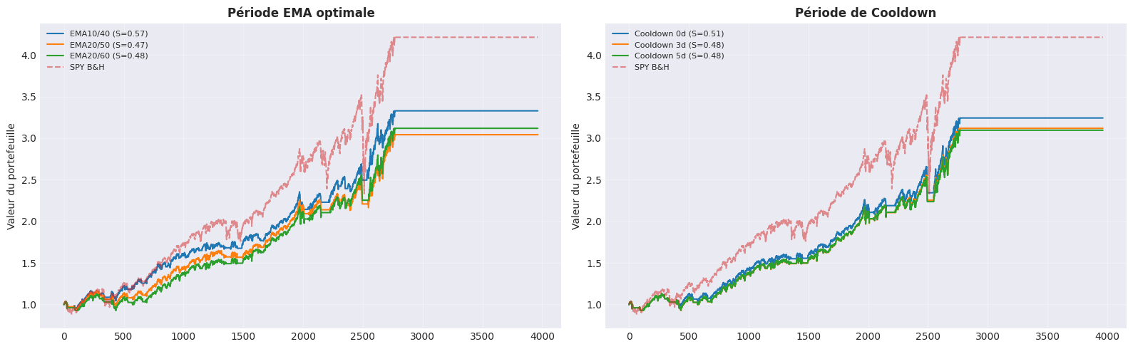
# Test différentes paires EMA = [10 , 40 ), "EMA10/40" ),20 , 50 ), "EMA20/50" ),20 , 60 ), "EMA20/60" ),print (f" { 'Période EMA' :<12} { 'Sharpe' :>8} { 'CAGR' :>8} { 'MaxDD' :>8} { 'Investi' :>8} " )print ("-" * 52 )= {}for (fast, slow), name in ema_pairs:= compute_ema(spy_close, fast)= compute_ema(spy_close, slow)= backtest_ema_cross_index(spy_close, ema_f, ema_s)= rprint (f" { name:<12} { r['sharpe' ]:>8.3f} { r['cagr' ]:>7.1%} { r['max_dd' ]:>7.1%} { r['pct_invested' ]:>7.1%} " )= max (ema_results.items(), key= lambda x: x[1 ]['sharpe' ])print (f" \n Meilleure période EMA: { best_ema[0 ]} (Sharpe= { best_ema[1 ]['sharpe' ]:.3f} )" )
Période EMA    Sharpe     CAGR    MaxDD  Investi
----------------------------------------------------
EMA10/40        0.572    7.9%  -10.6%   83.7%
EMA20/50        0.469    7.3%  -16.7%   75.5%
EMA20/60        0.483    7.5%  -17.9%   87.4%

Meilleure période EMA: EMA10/40 (Sharpe=0.572)
5. Test du Cooldown
# Test différentes valeurs de cooldown = [0 , 3 , 5 ]print (f" { 'Cooldown' :<10} { 'Sharpe' :>8} { 'CAGR' :>8} { 'MaxDD' :>8} " )print ("-" * 38 )= {}for cd in cooldowns:= backtest_ema_cross_index(spy_close, ema_fast, ema_slow, cooldown_days= cd)f" { cd} d" ] = rprint (f" { cd} j { '' :<7} { r['sharpe' ]:>8.3f} { r['cagr' ]:>7.1%} { r['max_dd' ]:>7.1%} " )= max (cooldown_results.items(), key= lambda x: x[1 ]['sharpe' ])print (f" \n Meilleur Cooldown: { best_cooldown[0 ]} (Sharpe= { best_cooldown[1 ]['sharpe' ]:.3f} )" )
Cooldown     Sharpe     CAGR    MaxDD
--------------------------------------
0j           0.509    7.8%  -15.3%
3j           0.483    7.5%  -17.9%
5j           0.478    7.4%  -17.7%

Meilleur Cooldown: 0d (Sharpe=0.509)
6. Test du Trailing Stop
def backtest_ema_with_trailing_stop(spy_close, ema_fast, ema_slow,= 3 ,= 0.95 ,= 0.05 ):""" Backtest EMA avec trailing stop. """ = [1.0 ]= False = 0 = None = None = 60 for i in range (warmup, len (spy_close)):= spy_close.iloc[i]= ema_fast.iloc[i]= ema_slow.iloc[i]if cooldown_counter > 0 :-= 1 # Check trailing stop if invested and entry_price and highest_since_entry:= max (highest_since_entry, price)= highest_since_entry * (1 - trailing_stop_pct)if price <= stop_price:= False = None = None = cooldown_days# EMA exit signal if fast_val < slow_val and invested:= False = None = None = cooldown_days# Entry signal elif fast_val > slow_val and not invested and cooldown_counter == 0 := True = price= price# Calculate return = (price / spy_close.iloc[i- 1 ]) - 1 if invested:= daily_return * position_sizeelse := 0 - 1 ] * (1 + port_return))# Métriques = np.diff(portfolio_values) / np.array(portfolio_values[:- 1 ])= pd.Series(portfolio_values[1 :], index= spy_close.index[warmup:])= (portfolio_values[- 1 ] / portfolio_values[0 ]) - 1 = len (returns) / 252 = (1 + total_ret) ** (1 / years) - 1 if years > 0 else 0 = np.std(returns) * np.sqrt(252 ) if len (returns) > 1 else 0 = (cagr - 0.03 ) / vol if vol > 0.001 else 0 = cum_returns.expanding().max ()= (cum_returns - running_max) / running_max= drawdown.min ()return {'cum' : cum_returns,'sharpe' : sharpe,'cagr' : cagr,'max_dd' : max_dd,'vol' : vol,'final_value' : portfolio_values[- 1 ]# Comparaison avec et sans trailing stop = backtest_ema_cross_index(spy_close, ema_fast, ema_slow)= backtest_ema_with_trailing_stop(spy_close, ema_fast, ema_slow)print (f" { 'Version' :<15} { 'Sharpe' :>8} { 'CAGR' :>8} { 'MaxDD' :>8} " )print ("-" * 43 )print (f" { 'Sans Trailing' :<15} { no_ts_result['sharpe' ]:>8.3f} { no_ts_result['cagr' ]:>7.1%} { no_ts_result['max_dd' ]:>7.1%} " )print (f" { 'Avec Trailing' :<15} { ts_result['sharpe' ]:>8.3f} { ts_result['cagr' ]:>7.1%} { ts_result['max_dd' ]:>7.1%} " )
Version           Sharpe     CAGR    MaxDD
-------------------------------------------
Sans Trailing      0.483    7.5%  -17.9%
Avec Trailing      0.805    9.9%  -13.8%
7. Comparaison avec SPY B&H
# EMA Crossover avec paramètres optimaux = backtest_ema_cross_index(spy_close, ema_fast, ema_slow)# SPY B&H = 60 = spy_close.iloc[warmup:] / spy_close.iloc[warmup]# Métriques SPY = spy_values.pct_change().dropna()= (spy_values.iloc[- 1 ] ** (252 / len (spy_values))) - 1 = spy_ret.std() * np.sqrt(252 )= (spy_cagr - 0.03 ) / spy_vol= (spy_values / spy_values.cummax() - 1 ).min ()print ("=== Comparaison vs SPY B&H ===" )print (f" { 'Stratégie' :<20} { 'CAGR' :>10} { 'Sharpe' :>10} { 'MaxDD' :>10} " )print ("-" * 53 )print (f" { 'EMA Crossover' :<20} { ema_result['cagr' ]:>9.1%} { ema_result['sharpe' ]:>10.3f} { ema_result['max_dd' ]:>9.1%} " )print (f" { 'SPY B&H' :<20} { spy_cagr:>9.1%} { spy_sharpe:>10.3f} { spy_dd:>9.1%} " )print (f" \n === Analyse du Beta ===" )# Beta du portefeuille par rapport à SPY = ema_result['cum' ].pct_change().dropna()= spy_values.pct_change().dropna()# Aligner les dates = port_returns.index.intersection(aligned_spy.index)if len (common_idx) > 100 := port_returns.loc[common_idx]= aligned_spy.loc[common_idx]= np.cov(port_aligned, spy_aligned)[0 , 1 ] / np.var(spy_aligned)print (f"Beta: { beta:.2f} " )print (f"Interprétation: { 'Signal-driven' if beta < 0.6 else 'Beta loading' if beta > 0.8 else 'Mixe' } " )
=== Comparaison vs SPY B&H ===
Stratégie                  CAGR     Sharpe      MaxDD
-----------------------------------------------------
EMA Crossover             7.5%      0.483    -17.9%
SPY B&H                   9.6%      0.454    -33.7%

=== Analyse du Beta ===
Beta: 0.43
Interprétation: Signal-driven
8. Visualisation des résultats
= plt.subplots(1 , 2 , figsize= (16 , 5 ))# Gauche: EMA periods comparison = axes[0 ]for name, r in ema_results.items():'cum' ].values, label= f" { name} (S= { r['sharpe' ]:.2f} )" , linewidth= 1.5 )= 'SPY B&H' , linestyle= '--' , alpha= 0.5 )'Période EMA optimale' , fontsize= 12 , fontweight= 'bold' )'Valeur du portefeuille' )= 8 )True , alpha= 0.3 )# Droite: Cooldown comparison = axes[1 ]for name, r in cooldown_results.items():'cum' ].values, label= f"Cooldown { name} (S= { r['sharpe' ]:.2f} )" , linewidth= 1.5 )= 'SPY B&H' , linestyle= '--' , alpha= 0.5 )'Période de Cooldown' , fontsize= 12 , fontweight= 'bold' )'Valeur du portefeuille' )= 8 )True , alpha= 0.3 )'ema_cross_index_analysis.png' , dpi= 150 , bbox_inches= 'tight' )print ("Graphique sauvegardé." )
9. Conclusions et recommandations
Résumé
Période EMA
(à remplir)
Cooldown
(à remplir)
Trailing Stop
(à remplir)
Sharpe
(à remplir)
CAGR
(à remplir)
Beta
(à remplir)
Verdict
Si Sharpe > 1.0: Déployer avec les paramètres optimaux
Points forts EMA Crossover SPY
Simplicité : Un seul signal (EMA cross) à suivreLiquidity : SPY est ultra-liquide, pas de slippageCooldown : Réduit les whipsaws et améliore la robustesseBeta faible : Signal-driven, pas juste beta loading
Limitations
Trend following : Ne fonctionne que en tendance (pas de range trading)Lag : EMA est un indicateur lagging (retard)Underperformance : En bull marché fort, peut sous-performer le B&H
Prochaines étapes
Déployer sur QC cloud avec les paramètres optimaux
Tester sur d’autres indices (QQQ, IWM, EFA)
Combiner avec un filtre de volatilité (VIX)
Explorer des variantes multi-timeframe (EMA daily + weekly)