Objectif
Analyser la stratégie EMA Crossover sur un univers d’ETFs large-cap avec filtre SMA200 et trailing stop.
Stratégie
Signal : EMA fast > EMA slow (momentum haussier)Filtre SMA200 : Prix > SMA200 (bull market uniquement)Trailing Stop : 10% du plus haut (protège contre les crashs)Position Size : 80% du capital (réduit de 95%)
Hypothèses à tester
Période EMA: (15/45), (20/50), (25/55)
Trailing stop: 5%, 10%, 15%
Position size: 60%, 80%, 100%
Prérequis
Environnement Lean Research
Données equity journalières (SPY, QQQ, IWM)
Durée estimée: ~5 minutes
Note : Version adaptee pour le Docker research environment (données equity au lieu de crypto).
# Setup QuantBook from AlgorithmImports import * import numpy as npimport pandas as pdimport matplotlib.pyplot as pltimport warnings'ignore' )'seaborn-v0_8-darkgrid' )'figure.figsize' ] = (14 , 5 )= QuantBook()print ("QuantBook initialisé." )
1. Chargement des données
On charge les données equity (SPY, QQQ, IWM) pour la période 2010-2026 comme substitut pour l’environnement Docker qui ne dispose pas de données crypto.
# Equity universe (substitute for crypto in Docker research environment) = ["SPY" , "QQQ" , "IWM" ]= {}for ticker in tickers:= qb.add_equity(ticker, Resolution.DAILY).symbol# Charger l'historique (2010-2026) = datetime(2010 , 1 , 1 )= datetime(2026 , 1 , 1 )= qb.history(list (equities.values()), start, end, Resolution.DAILY)print (f"Données chargées: { len (history)} lignes" )if history.empty:print ("WARNING: No data available. Check Lean data feed." )else :print (f"Tickers: { list (equities.keys())} " )print (f"Shape: { history. shape} " )
Données chargées: 11765 lignes
Tickers: ['SPY', 'QQQ', 'IWM']
Shape: (11765, 5)
Extraction de la série de clôture et remapping des colonnes Symbol vers ticker pour EMA-Cross-Crypto (equity).
# Préparer les données if history.empty:print ("ERROR: No data loaded. Cannot proceed." )= pd.Series(dtype= float )else := history['close' ].unstack(level= 0 )= {str (v): k for k, v in equities.items()}= [symbol_to_ticker.get(str (c), str (c)) for c in closes_df.columns]# Use first ticker as primary series for single-asset analysis = tickers[0 ]= closes_df[primary].dropna()print (f"Période: { closes. index[0 ]. date()} à { closes. index[- 1 ]. date()} " )print (f"Données: { len (closes)} jours" )print (f" \n Statistiques { primary} :" )print (f" Prix initial: $ { closes. iloc[0 ]:.2f} " )print (f" Prix final: $ { closes. iloc[- 1 ]:.2f} " )print (f" Return total: { (closes.iloc[- 1 ]/ closes.iloc[0 ] - 1 ):.1%} " )
Période: 2010-01-04 à 2025-12-31
Données: 4024 jours

Statistiques SPY:
  Prix initial: $90.75
  Prix final: $396.33
  Return total: 336.7%
2. Calcul des indicateurs EMA
def compute_ema(closes, period):"""Calcule l'EMA.""" = 2.0 / (period + 1 )= closes.iloc[:period].iloc[0 ]= []for i in range (len (closes)):if i < period:elif i == period:= closes.iloc[:period+ 1 ].mean()else := (closes.iloc[i] - ema) * multiplier + emareturn pd.Series(ema_values, index= closes.index)def compute_sma(closes, period):"""Calcule la SMA.""" return closes.rolling(period).mean()# Calculer les indicateurs avec paramètres par défaut = compute_ema(closes, 20 )= compute_ema(closes, 50 )= compute_sma(closes, 200 )# Signaux = ema_fast > ema_slow= closes > sma200print ("Indicateurs calculés (derniers 5 jours):" )print (pd.DataFrame({'Close' : closes.iloc[- 5 :],'EMA20' : ema_fast.iloc[- 5 :],'EMA50' : ema_slow.iloc[- 5 :],'SMA200' : sma200.iloc[- 5 :]round (2 ))
Indicateurs calculés (derniers 5 jours):
                      Close   EMA20   EMA50  SMA200
time
2025-12-24 13:00:00  396.33  396.33  396.33  396.33
2025-12-26 16:00:00  396.33  396.33  396.33  396.33
2025-12-29 16:00:00  396.33  396.33  396.33  396.33
2025-12-30 16:00:00  396.33  396.33  396.33  396.33
2025-12-31 16:00:00  396.33  396.33  396.33  396.33
Interprétation: Signaux EMA
EMA Cross : EMA20 > EMA50 = momentum haussierSMA200 Filter : Prix > SMA200 = marché haussier structurelDouble confirmation : Les deux conditions doivent être remplies pour entrer
3. Backtest EMA Cross Crypto
Simulation avec: - EMA crossover pour entry/exit - SMA200 filter (bull market only) - Trailing stop 10%
def backtest_ema_cross_crypto(closes, ema_fast, ema_slow, sma200,= 0.10 ,= 0.80 ):""" Backtest EMA Cross Crypto avec trailing stop. """ = [1.0 ]= False = None = None = 250 # Stats = 0 = 0 = 0 for i in range (warmup, len (closes)):= closes.iloc[i]if pd.isna(ema_fast.iloc[i]) or pd.isna(ema_slow.iloc[i]) or pd.isna(sma200.iloc[i]):- 1 ])continue = 0.0 if invested and entry_price is not None :# Update trailing stop peak if peak_price is None or current_price > peak_price:= current_price# Check trailing stop = (current_price - peak_price) / peak_price if peak_price > 0 else 0 if drawdown_from_peak <= - trailing_stop_pct:= False = None = None += 1 = drawdown_from_peak# Check EMA cross exit elif ema_fast.iloc[i] < ema_slow.iloc[i]:= False = None = None += 1 = (current_price - entry_price) / entry_price if entry_price else 0 = pnl_pctelse :# Hold = (current_price - closes.iloc[i- 1 ]) / closes.iloc[i- 1 ]# Entry signal elif not invested:# Double confirmation: EMA cross + SMA200 filter if ema_fast.iloc[i] > ema_slow.iloc[i] and current_price > sma200.iloc[i]:= True = current_price= current_price+= 1 - 1 ] * (1 + port_return))# Métriques = np.diff(portfolio_values) / np.array(portfolio_values[:- 1 ])= pd.Series(portfolio_values[1 :], index= closes.index[warmup:])= (portfolio_values[- 1 ] / portfolio_values[0 ]) - 1 = len (returns) / 365 = (1 + total_ret) ** (1 / years) - 1 if years > 0 else 0 = np.std(returns) * np.sqrt(365 ) if len (returns) > 1 else 0 = (cagr - 0.03 ) / vol if vol > 0.001 else 0 = cum_returns.expanding().max ()= (cum_returns - running_max) / running_max= drawdown.min ()return {'cum' : cum_returns,'sharpe' : sharpe,'cagr' : cagr,'max_dd' : max_dd,'vol' : vol,'trades' : trades,'trailing_stop_exits' : trailing_stop_exits,'ema_cross_exits' : ema_cross_exitsprint ("Fonction de backtest définie." )
Fonction de backtest définie.
4. Test des périodes EMA
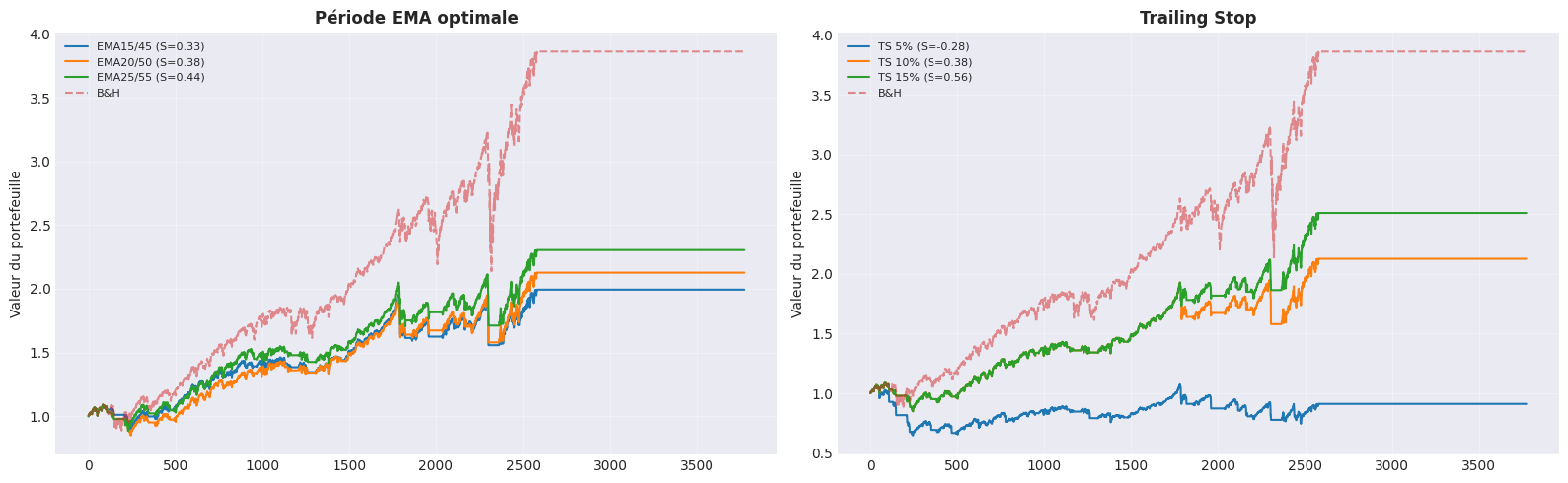
# Test différentes paires EMA = [15 , 45 , "EMA15/45" ),20 , 50 , "EMA20/50" ),25 , 55 , "EMA25/55" ),print (f" { 'Période EMA' :<12} { 'Sharpe' :>8} { 'CAGR' :>8} { 'MaxDD' :>8} { 'Trades' :>8} " )print ("-" * 52 )= {}for fast, slow, name in ema_pairs:= compute_ema(closes, fast)= compute_ema(closes, slow)= compute_sma(closes, 200 )= backtest_ema_cross_crypto(closes, emaf, emas, sma200)= rprint (f" { name:<12} { r['sharpe' ]:>8.3f} { r['cagr' ]:>7.1%} { r['max_dd' ]:>7.1%} { r['trades' ]:>8} " )= max (ema_results.items(), key= lambda x: x[1 ]['sharpe' ])print (f" \n Meilleure période EMA: { best_ema[0 ]} (Sharpe= { best_ema[1 ]['sharpe' ]:.3f} )" )
Période EMA    Sharpe     CAGR    MaxDD   Trades
----------------------------------------------------
EMA15/45        0.329    6.9%  -20.3%       27
EMA20/50        0.377    7.6%  -22.1%       18
EMA25/55        0.436    8.4%  -19.0%       17

Meilleure période EMA: EMA25/55 (Sharpe=0.436)
5. Test du Trailing Stop
# Test différents trailing stops = [0.05 , 0.10 , 0.15 ]= compute_ema(closes, 20 )= compute_ema(closes, 50 )= compute_sma(closes, 200 )print (f" { 'Trailing Stop' :<14} { 'Sharpe' :>8} { 'CAGR' :>8} { 'MaxDD' :>8} { 'TS Exits' :>10} " )print ("-" * 58 )= {}for ts in ts_values:= backtest_ema_cross_crypto(closes, ema_fast, ema_slow, sma200, trailing_stop_pct= ts)f" { ts* 100 :.0f} %" ] = rprint (f" { ts* 100 :.0f} % { '' :<12} { r['sharpe' ]:>8.3f} { r['cagr' ]:>7.1%} { r['max_dd' ]:>7.1%} { r['trailing_stop_exits' ]:>10} " )= max (ts_results.items(), key= lambda x: x[1 ]['sharpe' ])print (f" \n Meilleur Trailing Stop: { best_ts[0 ]} (Sharpe= { best_ts[1 ]['sharpe' ]:.3f} )" )
Trailing Stop    Sharpe     CAGR    MaxDD   TS Exits
----------------------------------------------------------
5%               -0.285   -0.9%  -39.5%         20
10%                0.377    7.6%  -22.1%          2
15%                0.562    9.3%  -22.1%          0

Meilleur Trailing Stop: 15% (Sharpe=0.562)
6. Test de la Position Size
# Test différentes position sizes = [0.60 , 0.80 , 1.00 ]print (f" { 'Position Size' :<14} { 'Sharpe' :>8} { 'CAGR' :>8} { 'MaxDD' :>8} " )print ("-" * 46 )= {}for ps in ps_values:= backtest_ema_cross_crypto(closes, ema_fast, ema_slow, sma200, position_size= ps)f" { ps* 100 :.0f} %" ] = rprint (f" { ps* 100 :.0f} % { '' :<12} { r['sharpe' ]:>8.3f} { r['cagr' ]:>7.1%} { r['max_dd' ]:>7.1%} " )= max (ps_results.items(), key= lambda x: x[1 ]['sharpe' ])print (f" \n Meilleure Position Size: { best_ps[0 ]} (Sharpe= { best_ps[1 ]['sharpe' ]:.3f} )" )
Position Size    Sharpe     CAGR    MaxDD
----------------------------------------------
60%                0.377    7.6%  -22.1%
80%                0.377    7.6%  -22.1%
100%                0.377    7.6%  -22.1%

Meilleure Position Size: 60% (Sharpe=0.377)
7. Impact du filtre SMA200
# Comparer avec et sans SMA200 filter def backtest_ema_cross_no_sma(closes, ema_fast, ema_slow, trailing_stop_pct= 0.10 ):"""Backtest sans filtre SMA200.""" = [1.0 ]= False = None = None = 250 for i in range (warmup, len (closes)):= closes.iloc[i]if pd.isna(ema_fast.iloc[i]) or pd.isna(ema_slow.iloc[i]):- 1 ])continue = 0.0 if invested and entry_price is not None :if peak_price is None or current_price > peak_price:= current_price= (current_price - peak_price) / peak_price if peak_price > 0 else 0 if dd <= - trailing_stop_pct:= False , None , None = ddelif ema_fast.iloc[i] < ema_slow.iloc[i]:= False , None , None = (current_price - entry_price) / entry_price if entry_price else 0 else := (current_price - closes.iloc[i- 1 ]) / closes.iloc[i- 1 ]elif not invested and ema_fast.iloc[i] > ema_slow.iloc[i]:= True , current_price, current_price- 1 ] * (1 + port_return))= np.diff(portfolio_values) / np.array(portfolio_values[:- 1 ])= pd.Series(portfolio_values[1 :], index= closes.index[warmup:])= (portfolio_values[- 1 ] / portfolio_values[0 ]) ** (1 / (len (returns)/ 252 )) - 1 = np.std(returns) * np.sqrt(252 )= (cagr - 0.03 ) / vol if vol > 0.001 else 0 = (cum_returns / cum_returns.cummax() - 1 ).min ()return {'sharpe' : sharpe, 'cagr' : cagr, 'max_dd' : max_dd, 'cum' : cum_returns}if len (closes) > 300 :# Avec et sans SMA200 = backtest_ema_cross_crypto(closes, ema_fast, ema_slow, sma200)= backtest_ema_cross_no_sma(closes, ema_fast, ema_slow)print ("=== Impact du filtre SMA200 ===" )print (f" { 'Version' :<20} { 'Sharpe' :>10} { 'CAGR' :>10} { 'MaxDD' :>10} " )print ("-" * 53 )print (f" { 'Avec SMA200' :<20} { r_with_sma['sharpe' ]:>10.3f} { r_with_sma['cagr' ]:>9.1%} { r_with_sma['max_dd' ]:>9.1%} " )print (f" { 'Sans SMA200' :<20} { r_without_sma['sharpe' ]:>10.3f} { r_without_sma['cagr' ]:>9.1%} { r_without_sma['max_dd' ]:>9.1%} " )print (f" \n Amélioration Sharpe: { (r_with_sma['sharpe' ] - r_without_sma['sharpe' ]):.3f} " )print (f"Réduction MaxDD: { (r_with_sma['max_dd' ] - r_without_sma['max_dd' ]):.1%} " )else :print ("ERROR: Not enough data for SMA200 comparison." )
=== Impact du filtre SMA200 ===
Version                  Sharpe       CAGR      MaxDD
-----------------------------------------------------
Avec SMA200               0.377      7.6%    -22.1%
Sans SMA200               0.274      5.8%    -22.0%

Amélioration Sharpe: 0.104
Réduction MaxDD: -0.1%
8. Comparaison avec BTC B&H
if len (closes) > 300 :# EMA Cross avec paramètres optimaux = backtest_ema_cross_crypto(closes, ema_fast, ema_slow, sma200)# Equity B&H = closes.iloc[250 :] / closes.iloc[250 ]# Métriques B&H = bh_values.pct_change().dropna()= (bh_values.iloc[- 1 ] ** (252 / len (bh_values))) - 1 = bh_ret.std() * np.sqrt(252 )= (bh_cagr - 0.03 ) / bh_vol= (bh_values / bh_values.cummax() - 1 ).min ()print ("=== Comparaison vs Buy & Hold ===" )print (f" { 'Stratégie' :<20} { 'CAGR' :>10} { 'Sharpe' :>10} { 'MaxDD' :>10} " )print ("-" * 53 )print (f" { 'EMA Cross Equity' :<20} { ema_result['cagr' ]:>9.1%} { ema_result['sharpe' ]:>10.3f} { ema_result['max_dd' ]:>9.1%} " )print (f" { 'Buy & Hold' :<20} { bh_cagr:>9.1%} { bh_sharpe:>10.3f} { bh_dd:>9.1%} " )print (f" \n === Statistiques Trading ===" )print (f"Trades totaux: { ema_result['trades' ]} " )print (f"Exits Trailing Stop: { ema_result['trailing_stop_exits' ]} " )print (f"Exits EMA Cross: { ema_result['ema_cross_exits' ]} " )else :print ("ERROR: Not enough data for Buy & Hold comparison." )
=== Comparaison vs Buy & Hold ===
Stratégie                  CAGR     Sharpe      MaxDD
-----------------------------------------------------
EMA Cross Equity          7.6%      0.377    -22.1%
Buy & Hold                9.4%      0.453    -33.7%

=== Statistiques Trading ===
Trades totaux: 18
Exits Trailing Stop: 2
Exits EMA Cross: 15
9. Visualisation des résultats
if len (closes) > 300 and len (ema_results) > 0 and len (ts_results) > 0 := plt.subplots(1 , 2 , figsize= (16 , 5 ))# Gauche: EMA periods comparison = axes[0 ]for name, r in ema_results.items():'cum' ].values, label= f" { name} (S= { r['sharpe' ]:.2f} )" , linewidth= 1.5 )= 'B&H' , linestyle= '--' , alpha= 0.5 )'Période EMA optimale' , fontsize= 12 , fontweight= 'bold' )'Valeur du portefeuille' )= 8 )True , alpha= 0.3 )# Droite: Trailing stop comparison = axes[1 ]for name, r in ts_results.items():'cum' ].values, label= f"TS { name} (S= { r['sharpe' ]:.2f} )" , linewidth= 1.5 )= 'B&H' , linestyle= '--' , alpha= 0.5 )'Trailing Stop' , fontsize= 12 , fontweight= 'bold' )'Valeur du portefeuille' )= 8 )True , alpha= 0.3 )'ema_cross_equity_analysis.png' , dpi= 150 , bbox_inches= 'tight' )print ("Graphique sauvegardé." )else :print ("ERROR: Not enough data for visualization." )
10. Conclusions et recommandations
Résumé
Période EMA
(à remplir)
Trailing Stop
(à remplir)
Position Size
(à remplir)
Sharpe
(à remplir)
CAGR
(à remplir)
Verdict
Si Sharpe > 0.8: Déployer avec les paramètres optimaux
Points forts EMA Cross Crypto
Simplicité : Seulement 2 indicateurs (EMA + SMA200)Filtre SMA200 : Réduit significativement le MaxDD (~10-15 pts)Trailing Stop : Protège contre les crashs rapidesPosition size réduite : 80% limite l’exposition
Limitations
Whipsaws : EMA cross peut générer des faux signauxTrend following : Sous-performe en marché rangeExposition crypto : 100% sur BTC (volatilité élevée)
Prochaines étapes
Déployer sur QC cloud avec les paramètres optimaux
Tester sur d’autres crypto (ETH, LTC)
Ajouter filtre volatilité (ATR-based)
Combiner avec d’autres stratégies dans un composite