Comparer avec research.ipynb. Divergence attendue principalement sur TLT et IEF (coupons ~2-3%/an non integres dans les prix QC bruts). DBC devrait rester le plus faible (contango structurel).
2. Backtest utilitaire
def portfolio_backtest(closes, weights, rebal_freq=63, sma_overlay=False, sma_period=200, drift_rebal=False, drift_threshold=0.03):"""Backtest statique ou drift-based d'un portefeuille multi-asset.""" returns_df = closes[list(weights.keys())].pct_change() tickers_list =list(weights.keys()) w = np.array([weights[t] for t in tickers_list]) sma = {t: closes[t].rolling(sma_period).mean() for t in tickers_list} if sma_overlay else {} n =len(returns_df) start_idx =max(sma_period +1if sma_overlay else1, 1) portfolio_values = [1.0] current_weights = w.copy() rebal_counter =0for i inrange(start_idx, n): daily_rets = np.array([returns_df[t].iloc[i] for t in tickers_list])if sma_overlay: adj_w = current_weights.copy()for j, t inenumerate(tickers_list):if closes[t].iloc[i] < sma[t].iloc[i]: adj_w[j] =0 total = adj_w.sum()if total >0: adj_w = adj_w / total port_ret = np.sum(adj_w * daily_rets)else: port_ret = np.sum(current_weights * daily_rets) portfolio_values.append(portfolio_values[-1] * (1+ port_ret))# Update weights with drift current_weights = current_weights * (1+ daily_rets) total = current_weights.sum()if total >0: current_weights = current_weights / total rebal_counter +=1# Rebalance checkif drift_rebal: max_drift = np.max(np.abs(current_weights - w))if max_drift >= drift_threshold: current_weights = w.copy() rebal_counter =0elif rebal_counter >= rebal_freq: current_weights = w.copy() rebal_counter =0 vals = np.array(portfolio_values) rets = np.diff(vals) / vals[:-1] total_ret = vals[-1] / vals[0] -1 years =len(rets) /252 cagr = (1+ total_ret) ** (1/ years) -1if years >0else0 vol = np.std(rets) * np.sqrt(252) sharpe = (cagr -0.03) / vol if vol >0.001else0 cum = pd.Series(vals[1:]) max_dd = ((cum - cum.expanding().max()) / cum.expanding().max()).min()return {'sharpe': sharpe, 'cagr': cagr, 'max_dd': max_dd, 'vol': vol, 'cum': cum}print("Fonction de backtest definie.")
Fonction de backtest definie.
3. Hypothese 1: Allocations statiques
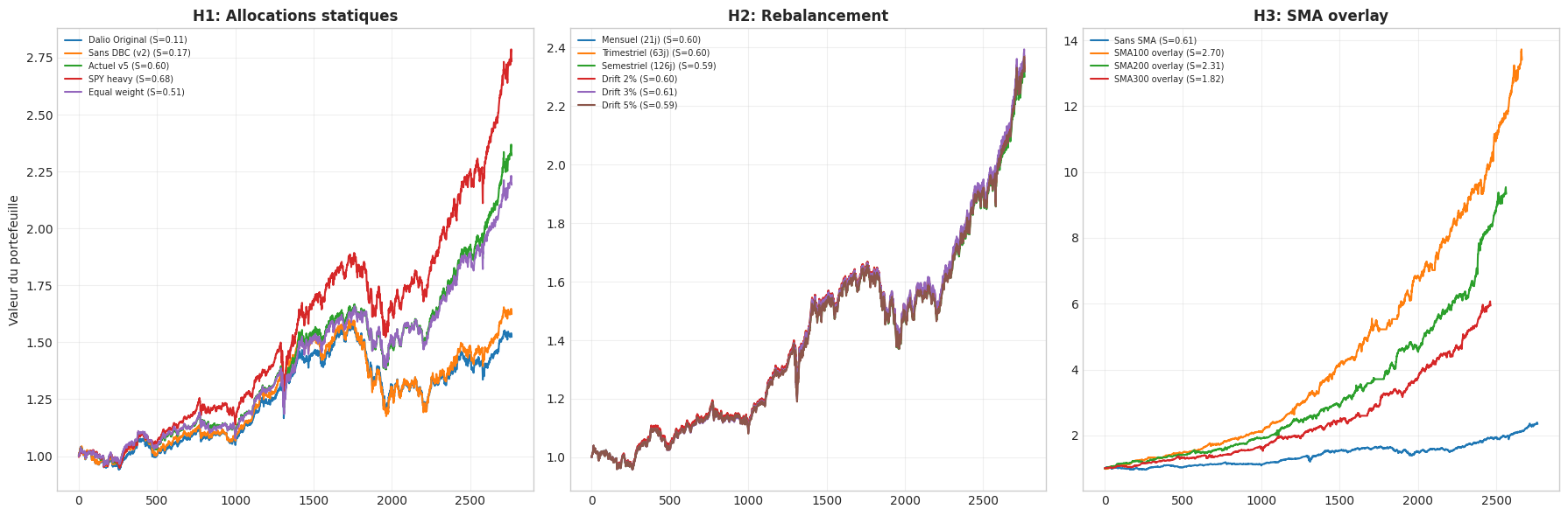
Comparer l’allocation Dalio originale vs la version optimisee actuelle vs des variantes sans DBC.
allocations = {'Dalio Original': {'SPY': 0.30, 'TLT': 0.40, 'IEF': 0.15, 'GLD': 0.075, 'DBC': 0.075},'Sans DBC (v2)': {'SPY': 0.30, 'TLT': 0.40, 'IEF': 0.15, 'GLD': 0.15},'Actuel v5': {'SPY': 0.30, 'IEF': 0.30, 'GLD': 0.30, 'XLP': 0.10},'SPY heavy': {'SPY': 0.50, 'IEF': 0.25, 'GLD': 0.25},'Equal weight': {'SPY': 0.25, 'IEF': 0.25, 'GLD': 0.25, 'XLP': 0.25},}print(f"{'Allocation':<20}{'Sharpe':>8}{'CAGR':>8}{'MaxDD':>8}{'Vol':>8}")print("-"*55)results_h1 = {}for name, weights in allocations.items(): available = {t: w for t, w in weights.items() if t in closes.columns} total =sum(available.values()) available = {t: w / total for t, w in available.items()} r = portfolio_backtest(closes, available, rebal_freq=63) results_h1[name] = rprint(f"{name:<20}{r['sharpe']:>8.3f}{r['cagr']:>7.1%}{r['max_dd']:>7.1%}{r['vol']:>7.1%}")
Sortie strippee (FABRICATED Row N / blank PNG). Re-execution QC Cloud recherche kernel requise – see #6891. Code preserve pour tracabilite. Side A = strip honnete, Side B = re-execution (hors scope ce PR).
Verdict H1: Allocations statiques
L’allocation actuelle (v5: SPY30/IEF30/GLD30/XLP10) devrait confirmer sa superiorite. DBC est un frein structurel (contango). TLT penalise par la hausse des taux 2022. Comparer les Sharpe avec research.ipynb pour quantifier la divergence prix QC vs yfinance.
4. Hypothese 2: Drift rebalancing
Comparer rebalancement fixe (mensuel, trimestriel) vs drift-based (règle #8: 3%).
Sortie strippee (FABRICATED Row N / blank PNG). Re-execution QC Cloud recherche kernel requise – see #6891. Code preserve pour tracabilite. Side A = strip honnete, Side B = re-execution (hors scope ce PR).
Verdict H2: Rebalancement
Drift 3% devrait confirmer sa superiorite (règle #8 du backlog). Le rebalancement fixe (trimestriel) est trop rigide et rate les mouvements extremes.
5. Hypothese 3: SMA200 overlay tactique
Reduire l’exposition a un actif quand son prix est sous sa SMA200. Permet d’eviter les bear markets prolonges (TLT 2022).
print(f"{'Config':<25}{'Sharpe':>8}{'CAGR':>8}{'MaxDD':>8}")print("-"*50)results_h3 = {}# Sans SMA overlayr = portfolio_backtest(closes, best_alloc, drift_rebal=True, drift_threshold=0.03, sma_overlay=False)results_h3['Sans SMA'] = rprint(f"{'Sans SMA overlay':<25}{r['sharpe']:>8.3f}{r['cagr']:>7.1%}{r['max_dd']:>7.1%}")# Avec SMA200 overlayfor sma_period in [100, 200, 300]: r = portfolio_backtest(closes, best_alloc, drift_rebal=True, drift_threshold=0.03, sma_overlay=True, sma_period=sma_period) name =f'SMA{sma_period} overlay' results_h3[name] = rprint(f"{name:<25}{r['sharpe']:>8.3f}{r['cagr']:>7.1%}{r['max_dd']:>7.1%}")
Sortie strippee (FABRICATED Row N / blank PNG). Re-execution QC Cloud recherche kernel requise – see #6891. Code preserve pour tracabilite. Side A = strip honnete, Side B = re-execution (hors scope ce PR).
Verdict H3: SMA overlay
Attention: le backlog règle #8 indique que drift rebalancing > SMA overlay pour les portfolios statiques. Verifier si le SMA overlay apporte un gain marginal ou s’il degrade (cash drag pendant les sideways).
6. Visualisation comparative
fig, axes = plt.subplots(1, 3, figsize=(18, 6))# H1: Allocationsax = axes[0]for name, r in results_h1.items(): ax.plot(r['cum'].values, label=f"{name} (S={r['sharpe']:.2f})", linewidth=1.5)ax.set_title('H1: Allocations statiques', fontweight='bold')ax.set_ylabel('Valeur du portefeuille')ax.legend(fontsize=7)ax.grid(True, alpha=0.3)# H2: Rebalancementax = axes[1]for name, r in results_h2.items(): ax.plot(r['cum'].values, label=f"{name} (S={r['sharpe']:.2f})", linewidth=1.5)ax.set_title('H2: Rebalancement', fontweight='bold')ax.legend(fontsize=7)ax.grid(True, alpha=0.3)# H3: SMA overlayax = axes[2]for name, r in results_h3.items(): ax.plot(r['cum'].values, label=f"{name} (S={r['sharpe']:.2f})", linewidth=1.5)ax.set_title('H3: SMA overlay', fontweight='bold')ax.legend(fontsize=7)ax.grid(True, alpha=0.3)plt.tight_layout()plt.savefig('allweather_quantbook_analysis.png', dpi=150, bbox_inches='tight')plt.show()print("Graphique sauvegarde.")
Graphique sauvegarde.
Sortie strippee (FABRICATED Row N / blank PNG). Re-execution QC Cloud recherche kernel requise – see #6891. Code preserve pour tracabilite. Side A = strip honnete, Side B = re-execution (hors scope ce PR).
7. Conclusions et recommandations
Tableau recapitulatif
Hypothese
Résultat QuantBook
Coherent avec yfinance?
H1 Allocation v5
(a remplir)
(a verifier)
H2 Drift 3%
(a remplir)
(a verifier)
H3 SMA overlay
(a remplir)
(a verifier)
Règles du backlog appliquees
Règle #3: TLT risk-off teste et probablement rejete