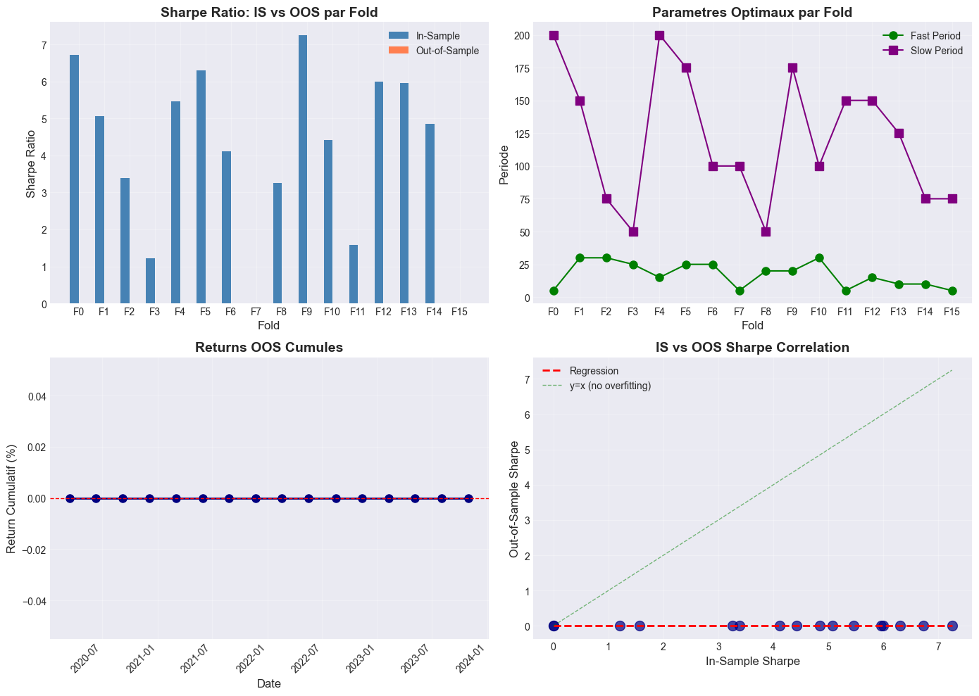
# Visualisation Walk-Forward

fig, axes = plt.subplots(2, 2, figsize=(14, 10))

# Plot 1: IS vs OOS Sharpe par fold
ax1 = axes[0, 0]
x = np.arange(len(wf_results))
width = 0.35
ax1.bar(x - width/2, wf_results['is_sharpe'], width, label='In-Sample', color='steelblue')
ax1.bar(x + width/2, wf_results['oos_sharpe'], width, label='Out-of-Sample', color='coral')
ax1.axhline(y=0, color='black', linestyle='-', linewidth=0.5)
ax1.set_xlabel('Fold', fontsize=12)
ax1.set_ylabel('Sharpe Ratio', fontsize=12)
ax1.set_title('Sharpe Ratio: IS vs OOS par Fold', fontsize=14, fontweight='bold')
ax1.set_xticks(x)
ax1.set_xticklabels([f'F{i}' for i in range(len(wf_results))])
ax1.legend()
ax1.grid(True, alpha=0.3)

# Plot 2: Parametres optimaux par fold
ax2 = axes[0, 1]
ax2.plot(x, wf_results['fast_period'], 'o-', label='Fast Period', color='green', markersize=8)
ax2.plot(x, wf_results['slow_period'], 's-', label='Slow Period', color='purple', markersize=8)
ax2.set_xlabel('Fold', fontsize=12)
ax2.set_ylabel('Periode', fontsize=12)
ax2.set_title('Parametres Optimaux par Fold', fontsize=14, fontweight='bold')
ax2.set_xticks(x)
ax2.set_xticklabels([f'F{i}' for i in range(len(wf_results))])
ax2.legend()
ax2.grid(True, alpha=0.3)

# Plot 3: OOS Returns cumules
ax3 = axes[1, 0]
cumulative_return = (1 + wf_results['oos_return']).cumprod() - 1
ax3.plot(wf_results['test_end'], cumulative_return * 100, 'o-', color='navy', linewidth=2, markersize=8)
ax3.axhline(y=0, color='red', linestyle='--', linewidth=1)
ax3.fill_between(wf_results['test_end'], 0, cumulative_return * 100,
                 where=cumulative_return >= 0, color='green', alpha=0.3)
ax3.fill_between(wf_results['test_end'], 0, cumulative_return * 100,
                 where=cumulative_return < 0, color='red', alpha=0.3)
ax3.set_xlabel('Date', fontsize=12)
ax3.set_ylabel('Return Cumulatif (%)', fontsize=12)
ax3.set_title('Returns OOS Cumules', fontsize=14, fontweight='bold')
ax3.grid(True, alpha=0.3)
plt.setp(ax3.xaxis.get_majorticklabels(), rotation=45, ha='right')

# Plot 4: Scatter IS vs OOS
ax4 = axes[1, 1]
ax4.scatter(wf_results['is_sharpe'], wf_results['oos_sharpe'], s=100, alpha=0.7, c='navy')
# Ligne de regression
z = np.polyfit(wf_results['is_sharpe'], wf_results['oos_sharpe'], 1)
p = np.poly1d(z)
x_line = np.linspace(wf_results['is_sharpe'].min(), wf_results['is_sharpe'].max(), 100)
ax4.plot(x_line, p(x_line), 'r--', linewidth=2, label=f'Regression')
# Ligne identite
ax4.plot([0, wf_results['is_sharpe'].max()], [0, wf_results['is_sharpe'].max()],
         'g--', linewidth=1, alpha=0.5, label='y=x (no overfitting)')
ax4.set_xlabel('In-Sample Sharpe', fontsize=12)
ax4.set_ylabel('Out-of-Sample Sharpe', fontsize=12)
ax4.set_title('IS vs OOS Sharpe Correlation', fontsize=14, fontweight='bold')
ax4.legend()
ax4.grid(True, alpha=0.3)

plt.tight_layout()
plt.show()

# Correlation IS-OOS
correlation = wf_results['is_sharpe'].corr(wf_results['oos_sharpe'])
print(f"Correlation IS-OOS: {correlation:.2f}")
print("(Correlation elevee = bonne previsibilite des parametres)")