Ce notebook demontre le workflow complet du pipeline ML : 1. Chargement des données OHLCV 2. Visualisation et exploration 3. Feature engineering 4. Entrainement des modèles (dry-run) 5. Evaluation des checkpoints sauvegardes
Pour un entrainement GPU complet , utiliser les scripts train_*.py en CLI.
import sysfrom pathlib import Path# Robust path setup: find scripts/ dir containing the pipeline modules # Walk up from CWD looking for scripts/train_classification.py as marker = []= Path.cwd()for _ in range (6 ):/ "scripts" )= _p.parent= None for c in _candidates:if (c / "train_classification.py" ).exists():= cbreak if _scripts_dir is None :raise FileNotFoundError ("Cannot find scripts/ directory with train_classification.py" )0 , str (_scripts_dir))import osimport numpy as npimport pandas as pdimport matplotlib.pyplot as pltprint ("Dependances chargees" )print (f"Scripts dir: { os. path. relpath(_scripts_dir)} " )
Dependances chargees
Scripts dir: scripts
1. Chargement des Données
Utilise les données telechargees via scripts/datasets/ ou des données synthetiques pour demo.
from data_utils import generate_synthetic_data, load_data, compute_data_hashfrom features import FeatureEngineer= Path("datasets/yfinance" )= "SPY" if data_dir.exists():= load_data(data_dir, symbol)print (f"Donnees reelles : { len (raw)} lignes, { raw. index. min (). date()} -> { raw. index. max (). date()} " )else := generate_synthetic_data(3000 )print (f"Donnees synthetiques : { len (raw)} lignes" )= FeatureEngineer(lookback= 20 )
Donnees synthetiques : 3000 lignes
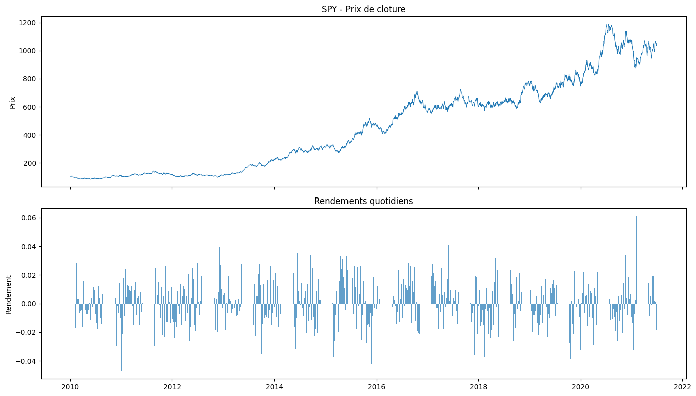
= plt.subplots(2 , 1 , figsize= (14 , 8 ), sharex= True )0 ].plot(raw.index, raw["Close" ], linewidth= 0.8 )0 ].set_title(f" { symbol} - Prix de cloture" )0 ].set_ylabel("Prix" )= raw["Close" ].pct_change().dropna()1 ].bar(returns.index, returns.values, width= 1 , alpha= 0.7 )1 ].set_title("Rendements quotidiens" )1 ].set_ylabel("Rendement" )print (f"Rendement moyen: { returns. mean():.5f} " )print (f"Volatilite annualisee: { returns. std() * np. sqrt(252 ):.4f} " )
Rendement moyen: 0.00089
Volatilite annualisee: 0.2353
2. Feature Engineering
Creation des features techniques : rendements multi-horizon, volatilite, RSI, MACD, Bollinger Bands.
= engineer.transform(raw)print (f"Features generees : { features. shape} " )print (f"Colonnes : { list (features.columns[:10 ])} ... ( { len (features.columns)} total)" )
Features generees : (2800, 38)
Colonnes : ['ret_1d', 'ret_5d', 'ret_10d', 'ret_20d', 'vol_5d', 'vol_20d', 'vol_ratio', 'ma_ratio_5', 'ma_ratio_10', 'ma_ratio_20']... (38 total)
count
2800.000000
2800.000000
2800.000000
2800.000000
2800.000000
2800.000000
2800.000000
2800.000000
2800.000000
2800.000000
...
2800.000000
2800.000000
2800.000000
2800.000000
2800.000000
2800.000000
2800.000000
2800.000000
2800.000000
2800.000000
mean
0.000964
0.004822
0.009666
0.019239
0.013968
0.014674
0.999189
1.001751
1.003979
1.008396
...
-43.826140
0.057989
0.023457
-0.061576
0.007988
0.008892
-0.000007
0.000028
0.000012
0.000969
std
0.014882
0.033078
0.046945
0.067487
0.005227
0.002425
1.126142
0.016195
0.024909
0.036899
...
29.912931
0.487368
1.035191
0.226107
0.002000
0.002180
0.020899
0.020846
0.021146
0.014879
min
-0.047170
-0.101775
-0.132353
-0.184494
0.000746
0.008295
0.018749
0.952037
0.926022
0.885417
...
-99.972674
-2.417940
-1.823116
-0.725784
0.002132
0.002949
-0.065017
-0.079824
-0.070392
-0.047170
25%
-0.009043
-0.017461
-0.022481
-0.027632
0.010187
0.012973
0.322231
0.990976
0.987478
0.983597
...
-69.497681
-0.253425
-0.669865
-0.214090
0.006632
0.007388
-0.014518
-0.013277
-0.013773
-0.009034
50%
0.000686
0.003672
0.007617
0.016559
0.013745
0.014678
0.632618
1.001807
1.003823
1.007208
...
-39.748085
0.072953
-0.197187
-0.063169
0.007904
0.008858
-0.000218
-0.000191
0.000246
0.000686
75%
0.010576
0.026435
0.040525
0.063236
0.017357
0.016275
1.236939
1.012604
1.019879
1.032145
...
-16.550693
0.360116
0.436605
0.098457
0.009236
0.010353
0.014015
0.013580
0.013952
0.010576
max
0.060981
0.126519
0.189904
0.259339
0.034367
0.024008
11.567945
1.057339
1.089759
1.124132
...
-0.051866
1.631855
8.441795
0.563215
0.014185
0.015060
0.079970
0.076515
0.081985
0.060981
8 rows × 38 columns
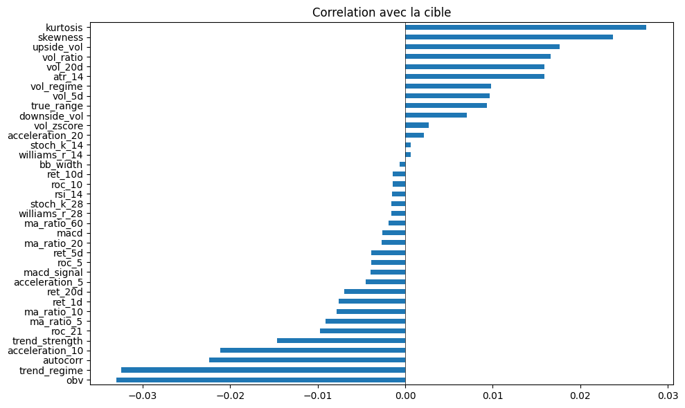
= "target" if target_col in features.columns:= features.corr()[target_col].drop(target_col).sort_values()= plt.subplots(figsize= (10 , 6 ))= "barh" , ax= ax)"Correlation avec la cible" )0 , color= "black" , linewidth= 0.5 )
3. Entrainement - Dry Run
Validation du pipeline avec données synthetiques. Pour un entrainement complet sur GPU, utiliser :
python scripts/train_lstm.py --data-dir ../datasets/yfinance --symbol SPY --hidden-size 512 --epochs 200
from train_classification import train_and_evaluate= generate_synthetic_data(500 )= engineer.transform(synth)= compute_data_hash(synth)# Binarize target: 1 if positive forward return, 0 otherwise "target" ] = (synth_features["target" ] > 0 ).astype(int )= train_and_evaluate(synth_features, model_type= "rf" , n_estimators= 50 , max_depth= 5 )print (f"RandomForest : Accuracy= { result_rf['metrics' ]['accuracy' ]} , F1= { result_rf['metrics' ]['f1' ]} " )
RandomForest : Accuracy=0.3333, F1=0.2234
from sequence_utils import build_sequences, normalize_sequencesfrom train_lstm import train_and_evaluate as train_lstm_model= engineer.transform(synth)= build_sequences(lstm_features, seq_len= 20 )= int (len (X) * 0.8 )= X[:split], X[split:]= y[:split], y[split:]= normalize_sequences(X_train, X_test)= train_lstm_model(X_train, y_train, X_test, y_test,= 64 , num_layers= 1 , epochs= 2 , batch_size= 32 , device= "cpu" )print (f"LSTM : MSE= { lstm_result['metrics' ]['mse' ]:.6f} , DirAcc= { lstm_result['metrics' ]['direction_accuracy' ]} " )
  Epoch 1/2  train=0.002215  val=0.000934  GPU=63C
  Epoch 2/2  train=0.001707  val=0.000878  GPU=63C
LSTM : MSE=0.001175, DirAcc=0.6071
4. Evaluation d’un Checkpoint
Chargement et evaluation d’un modèle sauvegarde. Requiert un checkpoint existant.
import json= Path("../checkpoints" )= []if ckpt_base.exists():for model_dir in ckpt_base.iterdir():if model_dir.is_dir():for ts_dir in model_dir.iterdir():if ts_dir.is_dir() and (ts_dir / "metadata.json" ).exists():= json.loads((ts_dir / "metadata.json" ).read_text())"path" : str (ts_dir), ** meta})if all_ckpts:= sorted (all_ckpts, key= lambda x: x["timestamp" ])[- 1 ]print (f"Checkpoint le plus recent : { latest['path' ]} " )print (f"Modele : { latest['model_type' ]} " )print (f"Metriques : { latest['metrics' ]} " )print (f"Data hash : { latest['data_hash' ]} " )else :print ("Aucun checkpoint trouve. Lancez un entrainement d'abord." )
Aucun checkpoint trouve. Lancez un entrainement d'abord.
5. Resume
Chargement données
OK
Feature engineering
OK
Dry-run classification
OK
Dry-run LSTM
OK
Checkpoint evaluation
A verifier après entrainement
Prochaines étapes : lancer les entrainements GPU complets via les scripts CLI.